Interferometry in Practice
References for today
- The Fourier Transform and its Applications by R. Bracewell
- Interferometry and Synthesis in Radio Astronomy by Thompson, Moran, and Swenson, particularly Appendix 2.1
- Essential Radio Astronomy by James Condon and Scott Ransom
This time
The punchline of today is that the complex-valued visibility function \(\mathcal{V}\) is the 2D Fourier transform of an image on the celestial sphere (with a small field of view)
$$ I(l, m) \leftrightharpoons \mathcal{V}(u, v) $$
and it is the visibility function that interferometers measure directly. The values of \(u, v\) for which interferometers are able to measure the visibility function depend on how the array of antennas is laid out and the spacing between them.
Most of today’s lecture will follow Chapters 2 and 3 of Interferometry and Synthesis in Radio Astronomy by Thompson, Moran, and Swenson. First, we will introduce a two-element interferometer and it’s response to a point source. Then, we’ll complexify this a bit to talk about an extended source (but still in 1D). Then, we’ll move on to discuss intensity distributions and the visibility function in the general case and then derive the relationship between \(I(l, m) \leftrightharpoons \mathcal{V}(u, v)\).
We’ll first develop the geometry and math of this relationship for small fields of view, so that you understand the result, at least in an abstract manner. Then we’ll spend the latter part of the course working through how a radio interferometer like the VLA or ALMA works to actually sample the visibility function.
R.A. and Dec
Let’s review our coordinates for images on the celestial sphere.
Declination’s the easier one, in my opinion. No matter where you are, if you move in declination, you move along a great circle (i.e., a circle that actually traces the circumference of the celestial sphere). We measure this in terms of 0 (celestial equator) to +90 degrees at the north celestial pole and -90 degrees at the southern celestial pole. You can split a degree into 60 arcminutes and an arcminute into 60 arcseconds.
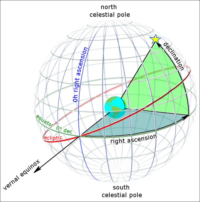
Credit: Sky and Telescope
Right Ascension is the one that sometimes trips me up. Because the sky rotates, we have this system of marking it using sidereal time: 24 hours of right ascension, sometimes broken up into 60 minutes, and 60 seconds. Although they are still in multiples of 60, these minutes and seconds we use for right ascension do not have the same angular size as arcminutes and arcseconds (even if we are on the celestial equator). For example, let’s say we have two points on the sky.
p1 = '00h42m00s', '+41d12m'
p2 = '00h42m01s', '+41d12m'
Same declination, but their R.A. values differ by one second. Can anyone guess how many arcseconds separate these points? The answer is about 11.3 arcseconds.
Usually, when we are talking about observing a smaller source (like a protoplanetary disk, or galaxy), we point in some direction towards that object and then define a small little postage stamp, commonly in units of \(\Delta \delta \) and \(\Delta \alpha \cos \delta\), in which case, the units describing the image are arcseconds. We’re still talking about spherical astronomy though, so this isn’t necessarily limited to small fields of view. We could have \(\Delta \delta\) be several degrees, for example.
TODO: Figure: point relative to center, and then Delta directions coming off of it.
Direction cosines
In a moment, we’re going talk about the mechanics of interferometers observing the celestial sphere and how these relate to Fourier transforms. Before we talk about that, though, there’s a concept I want to introduce while we’re still talking about units for images.
Practically speaking, most images we might make with ALMA or the VLA will have a small field of view (< 1 arcminute). In this regime, it simplifies a lot to talk about “flat” images, i.e., image planes that are tangent to the field center. In 1D, it would look like this
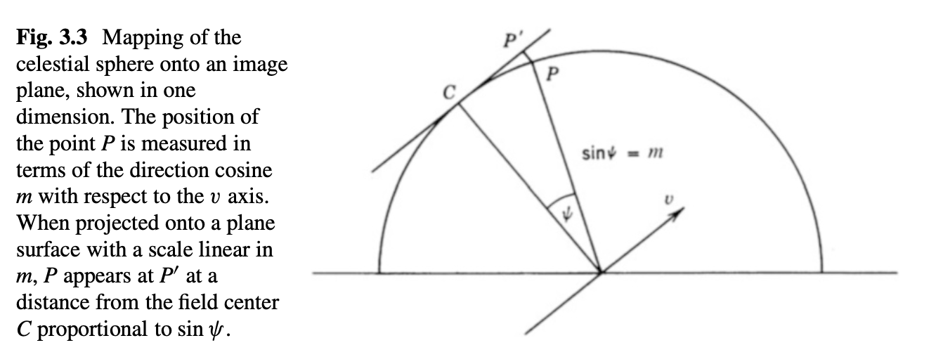
The concept of the direction cosine. Credit: Fig 3.3 TMS
The direction cosines are $$ l = \sin(\Delta \alpha \cos \delta) $$ and $$ m = \sin(\Delta \delta) $$ relative to the phase center. You can see from the figure that it is the direction cosine that is actually tracking the position on the tangent plane, where we are defining our image. I know I just wrote down \(\sin\) but I called these direction cosines. The term comes about from the way you’d set up the problem in two dimensions, where you might use cosine of the complementary angle instead, but it’s just a matter of convention.
Because they are outputs from trigonometric functions, they are technically unitless. Though l and m are technically unitless and measures of linear distance, for small angular extent, they could also be considered to have units of radians. So it will be common that we refer to $$ l = \sin(\Delta \alpha \cos \delta) \approx \Delta \alpha \cos \delta $$ and $$ m = \sin(\Delta \delta) \approx \Delta \delta. $$
This probably sounds pointless, since we just arrived back at the same units we started with. Hopefully the reasons why we might wish to use these units will become apparent after we cover more about the interferometer. And remember that you can always exactly convert from direction cosine back to angular usits (e.g. \(\Delta \alpha \cos \delta\)) by doing \(\sin^{-1}\), it’s just that for most small angles we’ll be dealing with, this operation is essentially an identity function. All of this goes out the window when we consider wide-field imaging (which we won’t have time to talk about in this course, unfortunately).
Introduction to a 2-element interferometer
Consider this geometric situation
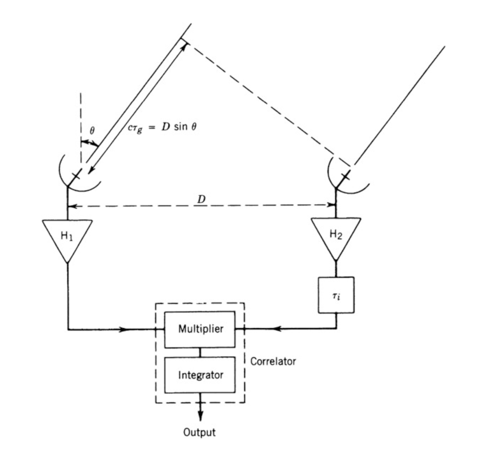
Credit: TMS Fig 2.1
The antennas are spaced directly east-west, and they are observing a source in the far-field, i.e., the radiation from a distant cosmic source appears as a plane wave. First, we will consider the case of a point-source; later we will extend this formalism to spatially extended sources. We’ll assume the primary beam of each antenna is large, such that they can observe radiation from a source located a wide range of \(\theta\) angles. We’ll assume that we’re observing in a narrow slice of frequency around \(\nu\), essentially monochromatic.
The wavefront from the source arrives at the right antenna some time $$ \tau_g = \frac{D}{c} \sin \theta $$ before it reaches the left one. This is called the geometric time delay.
Each antenna has its own signal voltage stream: $$ V_1 = \sin 2 \pi \nu t $$ and $$ V_2 = \sin 2 \pi \nu (t - \tau_g). $$
These streams are multiplied together in a correlator and then time-averaged over some interval. The output of the correlator is proportional to $$ F(t, \tau_g) = \sin (2 \pi \nu t) \sin 2 \pi \nu (t - \tau_g), $$ which we can expand using our trig sum identities for sine to $$ F(t, \tau_g) = \sin^2(2 \pi \nu t) \cos(2 \pi \nu \tau_g) - \sin(2 \pi \nu t)\cos(2 \pi \nu t) \sin(2 \pi \nu \tau_g). $$
We can simplify this equation based on our knowledge that the correlator multiplies and then adds (integrates, typically for a few seconds).
- The central frequency \(\nu\) is on the order of 10s of MHz to nearly a THz
- \(\theta\) (baked into \(\tau_g\)) is rotating at the Earth’s rotational velocity, which is \(10^{-4}\;\mathrm{rad\,s}^{-1}\).
- \(D\) must be smaller than \(10^7\;\)m for terrestrial baselines
This means that the rate of variation of \(\nu \tau_g \ll \nu t\) by several orders of magnitude.
So long as our averaging interval is \(T \gg 1/\nu\) (which is satisfied by a typical multi-second integration), $$ \langle \sin^2 (2 \pi \nu t) \rangle = 1/2 $$ and $$ \langle \sin(2 \pi \nu t)\cos(2 \pi \nu t) \rangle = 0 $$ so we’re left with $$ F \propto \cos (2 \pi \nu \tau_g). $$ We can also define \(l = \sin \theta\) and then we can write $$ F \propto \cos (2 \pi \nu \tau_g) = \cos \left (\frac{2 \pi D l}{\lambda} \right ). $$
This is called the fringe function of a two-element interferometer
TODO: draw as a linear relationship vs. \(l\), i.e., an oscillating sine wave TODO: then include the fringe plot itself
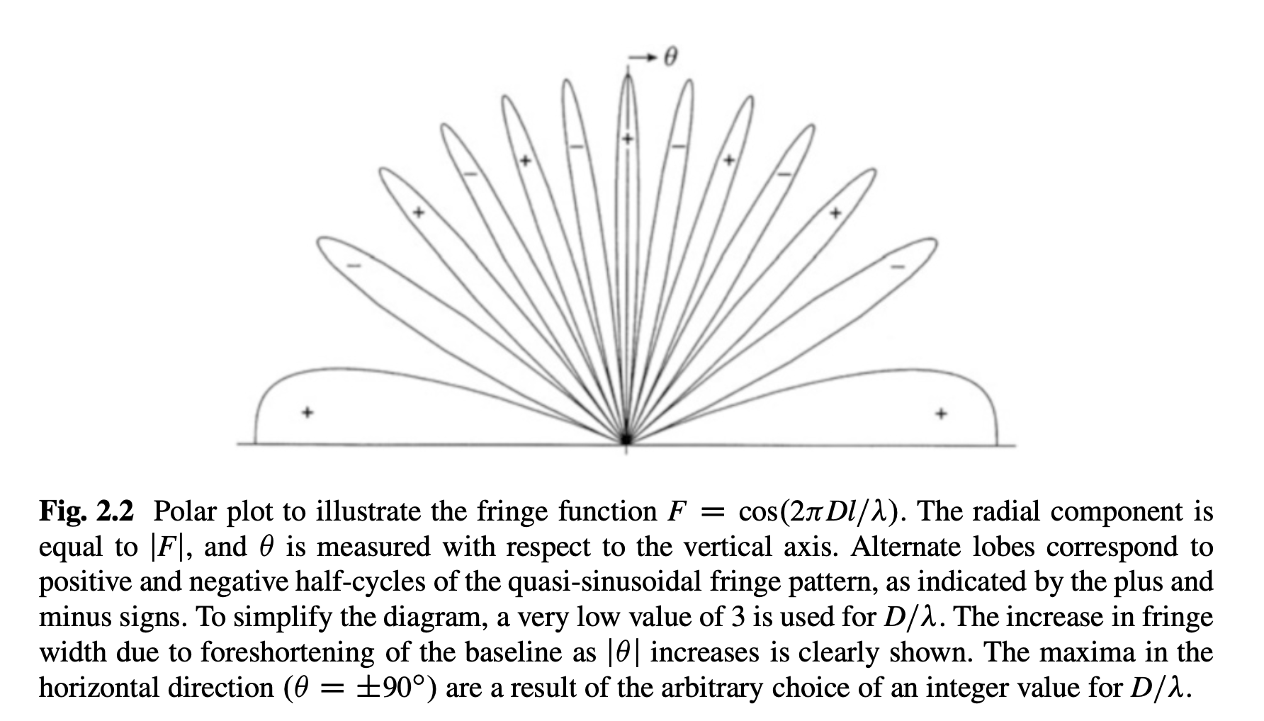
The fringe function (plotted here as \(|F|\)) can be thought of as the directional power pattern of the interferometer in the case the antennas are isotropic. Credit: TMS Fig 2.2
So, you see that the 2-element interferometer has a sine/cosine sensitivity to the sky along the east-west axis. It has no sensitivity along the north-south direction.
2-element interferometer for a spatially resolved source
Now we’ll consider a slightly more complex interferometer.
- The antennas are (somewhat) directional
- They track the source as it moves across the sky, from the rotation of the Earth. This introduces an instrumental time delay
$$ \tau_i = \frac{D}{c} \sin \theta_0. $$ I.e., this keeps the waveforms in sync so long as we’re looking directly at \(\theta_0\).
The direction the antennas are pointed is called the phase reference position, which we’ll denote as \(\theta_0\) and tracks the source as it rotates across the sky.
TODO: make a figure showing \(\Delta \theta\) offset.
And let us consider radiation from a direction \(\theta_0 - \Delta \theta\), where \(\Delta \theta\) is a small angle. As before, the fringe response term is $$ \cos (2 \pi \nu \tau) = \cos \left \{ 2 \pi \nu \left [ \frac{D}{c} \sin (\theta_0 - \Delta \theta) - \tau_i \right ] \right \}. $$ Using the sine formulas for difference and simplifying with \(\cos \Delta \simeq 1\) for small angles, we have $$ \cos (2 \pi \nu \tau) \simeq \cos \left [ 2 \pi \nu \frac{D}{c} \sin \Delta \theta \cos \theta_0 \right]. $$
Let’s stare at this equation a bit more. Assuming we’re holding observing frequency fixed, the angular resolution of the fringes is determined by the projected length of the baseline orthogonal to the direction of the source, which is \(D \cos \theta_0\). This is a pretty ordinary physical measurement of a distance, i.e., we would measure it to be something like 50 meters.
Of course, observing frequency also makes a difference. If we’re observing at higher frequencies (shorter \(\lambda\)), the fringe resolution is going to better (this is just another form of the \(\lambda/D\) resolution relationship for telescopes showing up).
So, we can define a new variable for this projected baseline length $$ u = \frac{D \cos \theta_0}{\lambda} = \frac{\nu_0 D \cos \theta_0}{c}. $$ \(u\) is the number of wavelengths (at that observing wavelength) that are needed to span the projected baseline length. It is measured in multiples of “\(\lambda\),” i.e., you might see a baseline length described as \(u = \) 300 kilolambda. \(u\) is called a spatial frequency.
Now we will redefine our sky coordinate variable \(l = \sin \Delta \theta\), and we find that we can write the fringe response as $$ F(l) \propto \cos (2 \pi \nu_0 \tau) \propto \cos (2 \pi u l). $$
If \(u\) gets larger (either by moving the antennas further apart and increasing the projected baseline, or by observing at a higher frequency), then the spatial resolution (spacing of the fringes) will get better.
We see that the quantity \((ul)\) appears inside of a trigonometric function, so this means the quantity must be dimensionless.
This motivates the many different ways we can think about these variables in the image plane and the visibility domain.
Unitless
The first way is to recognize that
- \(l\) is technically unitless, since it is \(\sin(\Delta \theta)\)
- \(u\) itself is also technically unitless, it’s just the baseline length measured in a number of wavelengths (e.g., kilolambda)
- Inside this \(\cos\) term, though, \(u\) plays the role of a frequency, i.e., “cycles per unit \(l\)”
Both of these variables do correspond to actual distances, the interferometer does have some baseline, which corresponds to its ability to resolve a source of some actual size on the sky. It’s just with this way of thinking about it, we measured both of those sizes using dimensionless units (and that’s OK)!
Unitful
We can put a little bit more sense to this by bringing back the small angle approximation, and saying that because \(\Delta \theta\) is small, then \(l = \sin \Delta \theta \approx \Delta \theta\), and so it is as if we measured \(l\) in some angular unit, like radians or arcseconds.
- If \(l\) is small, then we would say that it can be measured in radians (which can then be converted to arcseconds)
- Then \(u\) is measured in cycles/radian or cycles/arcsec
Because of this small angle approximation for the interferometer geometry, it allows us to equate “multiples of lambda” to “cycles per angle” as a spatial frequency.
Let’s walk through an example, and say that we’re observing a
- do small angle approximation to say l in units of radians
- convert to u
TODO: redraw waveform. This makes a lot of sense if you just draw the waveform up on the sky.
Compared to last time, we now assumed some directional sensitivity for each antenna, such as this power pattern
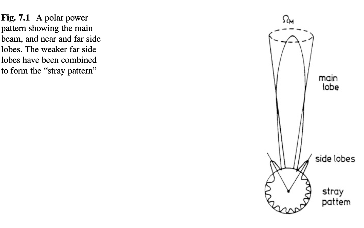
Credit: Tools of Radio Astronomy, Fig 7.1
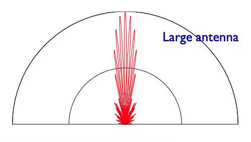
The fringe pattern modified by the antenna power pattern. Credit: Rick Perley’s slides, NRAO summer synthesis imaging school 2022.
Recap: so now we’ve redefined the fringe function to talk about the response to a spatially resolved source, as a function of projected baseline length. And, we’ve introduced the concept of spatial frequency.
Fourier transform relationship
We just derived and drew the fringe function as the response of the interferometer on the sky and examined how it changes as we change the position of the antennas on the ground. The essential response \(R(l)\) of the interferometer to some sky distribution \(I(l)\) is to act as a convolution $$ R(l) = \cos(2 \pi u l) * I(l) $$
Another way to look at this is to consider the Fourier pair of the fringe function when the antennas are at a fixed (instantaneous) baseline distance \(u_0\), $$ \cos(2 \pi u_0 l) \leftrightharpoons \frac{1}{2} [\delta(u + u_0) + \delta(u - u_0)]. $$
Let us define the visibility function \(\mathcal{V}(u)\) as the Fourier transform of the sky brightness distribution (the true one)
$$ I(l) \leftrightharpoons \mathcal{V}(u). $$ \(\mathcal{V}(u)\) represents the amplitude and phase of the sinusoidal component of the intensity distribution with spatial frequency \(u\) cycles per radian.
Then, we can bring out our old friend the multiplication/convolution algorithm. $$ \cos(2 \pi u l) * I(l) \leftrightharpoons \frac{\mathcal{V}(u)}{2} [\delta(u + u_0) + \delta(u - u_0)]. $$