Collisional Processes
References for this lecture
- Draine Ch. 2 (primary)
Intro
Collisions are one of the main ways in which energy is transferred about the ISM, so in order to understand the physics of the ISM, we need to understand the physics of collisions.
- thermal, electrical, diffusion coefficients
- produce most excitations of atoms and molecules (which then emit photons)
- recombine ions + electrons
- chemical reactions
Goal: set up a basic physical framework for understanding different types of collisions, and how their rates depend on density and temperature.
Types of collisional interactions and how we’ll understand them
- long range Coulomb (charges, ions, etc…) \(\propto 1/r\) potential: impact approximation
- intermediate range \(\propto r^{-4}\) potential induced dipole between ions and neutral atoms or molecules: scattering by \(\propto r^{-4}\) potential
- interactions between electrons and neutrals: experimental data
- short-range interactions between neutrals: “hard-sphere” estimates
Collisional rates and rate coefficients
Consider a general two-body collisional process
$$ A + B \rightarrow \mathrm{products}. $$
We can write the (average) reaction rate per unit volume (units \(\mathrm{cm}^{-3} \mathrm{s}^{-1}\)) as
$$ n_A n_B \langle \sigma v \rangle_{AB} $$
i.e., the rate is proportional to the number density of each species and the two-body collisional rate coefficient, \( \langle \sigma v \rangle_{AB} \), which has units of \(\mathrm{cm}^3 \mathrm{s}^{-1}\). Once you know the rate coefficient, this is a pretty simple relationship, just multiplying terms together. But let’s unpack how we calculate the rate coefficient.
How do we calculate this coefficient?
First, let’s consider the cross-section of the reaction
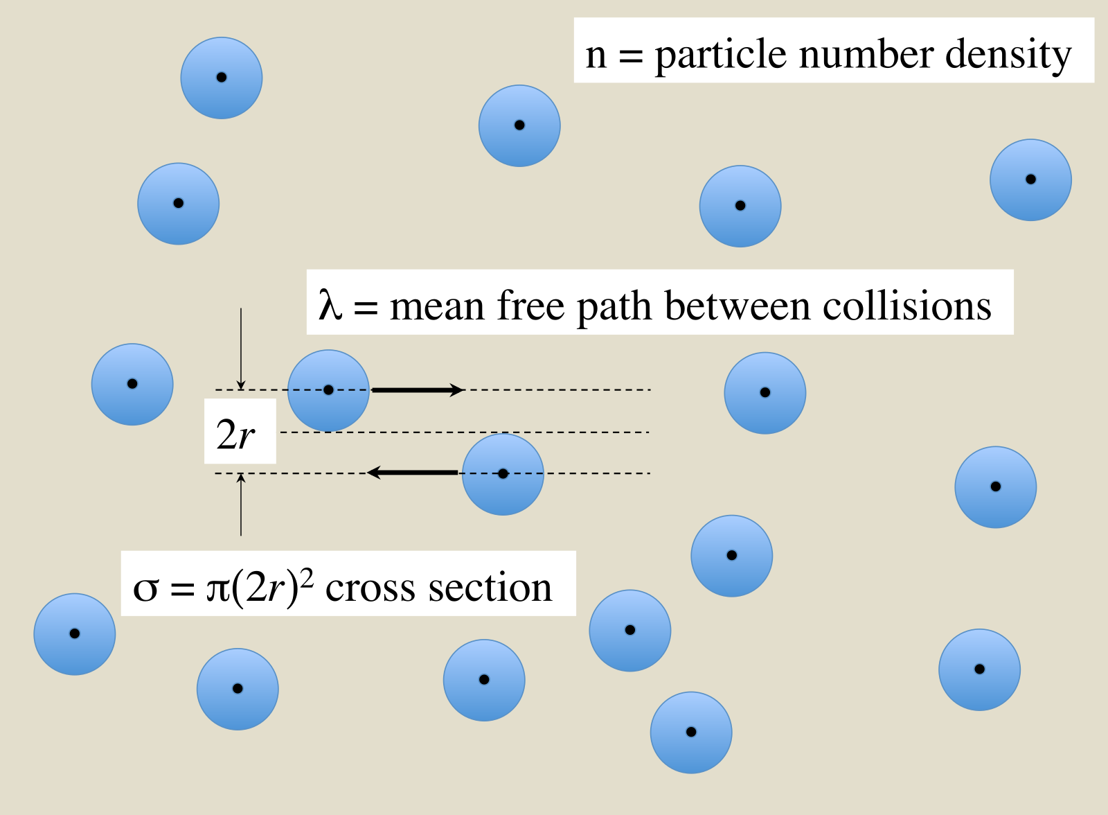
Scattering Cross Section. Attribution: Wikipedia: Qwerty123uiop
$$ \sigma = \frac{1}{n \lambda} $$
where \(n\) is number density and \(\lambda\) is the mean free path. Generally, \(\sigma \) can be thought of as the cross-sectional area (hence the name) for the interaction, and it has units of area (\(\mathrm{cm}^2\)), just like a cross-section of a solid. I.e., if the cross-section of the spheres are larger, then they’re more likely to hit each other (interact). However, if the cross-section is very small, it’s unlikely that they’ll hit each other (interact).
For the types of interactions we’re talking about, the cross-section of the interaction can be dependent on the relative velocity between the particles, \(\sigma(v)\).
For a gas, what can we generally say about the distribution of velocities of the particles? For a fluid in thermal equilibrium, the distribution function of the relative speed of encounters between particles is given by a Maxwellian velocity distribution
$$ f_v \, \mathrm{d}v = 4 \pi \left (\frac{\mu}{2 \pi k_B T }\right)^{3/2} \exp(- \mu v^2/2 k_B T) \, v^2 \mathrm{d} v $$
where $$ \mu = \frac{m_A m_B}{m_A + m_B} $$ is the reduced mass of the collisional partners. \(f_v\) is a distribution function, so to find the fraction of encounters that have relative speeds \(v_a < v < v_b\), we would just need to integrate over the relevant range $$ \int_{v_a}^{v_b} f_v \, \mathrm{d}v, $$ and to find the average value (i.e., expectation value) of some quantity \(X(v)\), we’d do $$ \langle X \rangle = \int_{0}^{\infty} X(v) f_v \, \mathrm{d}v. $$
Getting back to the original goal, we want to calculate the two-body collisional rate coefficient, \( \langle \sigma v \rangle_{AB} \), where \(X = \sigma v \). The cross section \(\sigma\) is a function of velocity \(\sigma(v)\), so we have \(X = \sigma(v) v \), or $$ \langle \sigma v \rangle_{AB} = \int_0^\infty \sigma_{AB}(v) v f_v \, \mathrm{d}v. $$
Following Draine (S2.1), we can also do a change of variables to center of mass energy \(E = \mu v^2/2\) to make the calculations more convenient.
Three-body collisions may be important in some situations, such as for populating the high-\(n\) levels of hydrogen. Their reaction rate is $$ k_{ABC} n_A n_B n_C $$ where \(k_{ABC}\) is the three-body collisional rate coefficient.
Inverse-Square Law Forces
Let’s consider the scattering by two particles interacting through an inverse square law \(1/r^2\), called Rutherford or Coulomb Scattering.
Question time
- How can we quickly get an estimate of the momentum transferred between two particles when they interact?
- What are some quick ways we could estimate this? If we needed to be very accurate, what would we need to do?
Impact approximation
A proper treatment involves some tedious integrals (see the Wikipedia article for reference), but we can get to an order-of-magnitude estimate using the “impact approximation.”
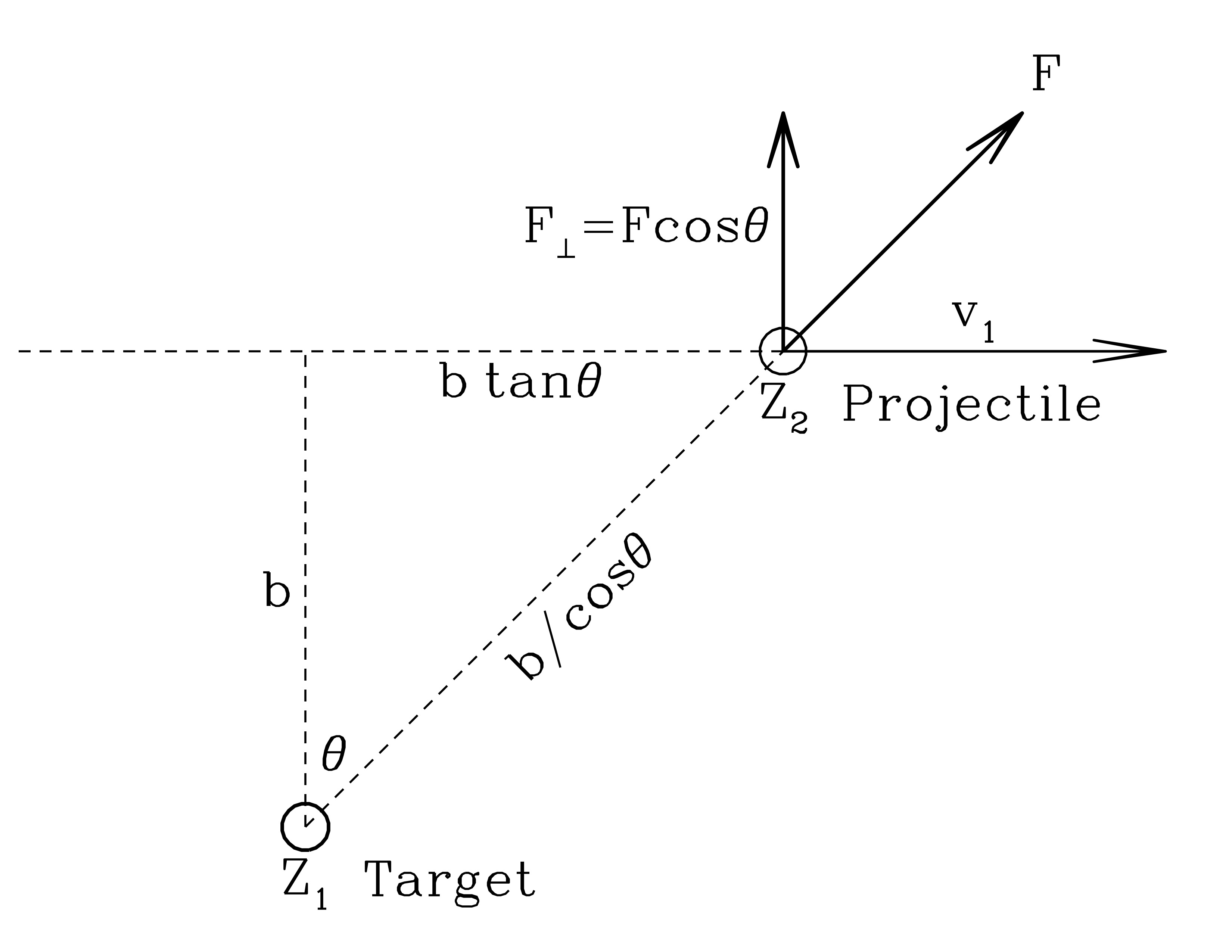
Coordinates for the Impact Approximation. Attribution: Draine Figure 2.1
Coulomb force
$$ F_{12} = \frac{Z_1 Z_2 e^2}{r^2} $$
Super simple way
Change in momentum is an impulse, $$ \Delta p = F \Delta t = m \Delta v. $$ And we’ll calculate the impulse given by the product of the perpendicular force at closest approach times the characteristic interaction time. This is likely to be the “most wrong” calculation, but it should at least get us in the ball park in terms of order of magnitude.
The instantaneous force perpendicular to the trajectory is $$ F_\bot = \frac{Z_1 Z_2 e^2}{(b \cos \theta)^2} \cos \theta = \frac{Z_1 Z_2 e^2}{b^2} \cos^3 \theta $$
What is “characteristic time” for the interaction? A decent guess is \(b/v_1\). Then the change in momentum is just
$$ \Delta p = \frac{Z_1 Z_2 e^2}{b v_1}. $$
A (slightly) more thorough treatment in the textbook (Draine 2.2.1) yields a more accurate $$ \Delta p = 2 \frac{Z_1 Z_2 e^2}{b v_1}. $$
Great, how can we use this to estimate things relevant to the ISM, such as the ionization rate of an atom with a single bound electron?
Collisional Ionization
Let \(I\) be the energy required to ionize the atom, i.e., completely unbind the electron.
We will consider the ionizer to be (another) electron that is moving fast enough such that its kinetic energy is \(\gg I\). If we could directly translate this energy to unbinding the electron, it would. But, we’re considering glancing (and more distant) interactions, so it’s not immediately clear how much we’d transfer.
If \(b\) is small, more energy will transferred. If \(b\) is large, less energy will be transferred. There will be some \(b\) so large that an insufficient amount of energy will be transferred to unbind the electron and ionize the atom. Let’s use our impact approximation to calculate this.
The criterion is $$ \frac{(\Delta p)^2}{2 m_e} > I $$ i.e., transfers of momentum exceedingFy the ionization energy.
We use this and the \(\Delta p\) equation above to solve for a maximum impact parameter
$$ b_\mathrm{max} = \left [ \frac{2 Z_p^2 e^4}{m_e v^2 I} \right ]^{1/2} $$
We can use the impact parameter as the “radius” of the cross-section, therefore the cross-section area for an ionizing interaction is $$ \sigma(v) \approx \pi b_\mathrm{max}^2(v). $$
Now we calculate the thermal rate coefficient $$ \langle \sigma v \rangle = \int_{v_\mathrm{min}}^\infty \sigma(v) v f_v \, \mathrm{d}v. $$ \(f_v\) is still given by the Maxwellian distribution, so we have $$ \langle \sigma v \rangle = Z_p^2 \left (\frac{8 \pi}{m_e kT} \right)^{1/2} \frac{e^4}{I}e^{-I/kT}. $$
For a hydrogen atom, the ionization energy is $$ I = \frac{13.602}{n^2} \, [\mathrm{eV}] $$ where \(n\) is the principal quantum number. For highly excited energy (\(n \approx 100\)), the ionization energy becomes small and the collisional ionization rate becomes very large.
Electron-ion inelastic scattering: Collisional strength \(\Omega_{ul}\)
We just discussed elastic scattering of electrons by ions, whereby momentum transfer between the two is dominated by “distant” encounters with impact parameters much larger than the relevant scales of the atom.
When the fast-moving electron does pass very close to the atom with bound electron, however, quantum mechanics plays a role (as it always does…) and the bound electron may transition to another energetically allowed state.
It’s common to write the cross-section for these interactions using a dimensionless quantity \(\Omega_{ul}\) called the collision strength. You can see S 2.3 of Draine for the full details, but the important part is that $$ \langle \sigma v \rangle_{u \rightarrow l} \propto \frac{\Omega_{ul}}{g_u \sqrt{T}}. $$ The good news is that
- \(\Omega_{ul}\) is approximately indepedent of \(T\) for temperatures below 10,000 K
- typical values of \(\Omega_{ul}\) are 1 - 10
- this means collisional rate coefficient \(\langle \sigma v \rangle_{u \rightarrow l}\) is \(\propto T^{-1/2}\)
Inelastic collisions play a role in line radiation from hot gas, since they leave the atom in an excited state, from which it decays by emitting a photon.
Ion-Neutral Collision Rates
A charged ion particle (more than just an electron) interacting with neutral particles (atoms or molecules). If the two are separated by more than a few Å, the charged particle creates an electric field \(\vec{E}\) which polarizes the neutral.
In the case of a simple hydrogen atom, you can think of this as the proton and electron moving to separate sides. The neutral acquires a dipole moment \(\vec{P} = \alpha_N \vec{E}\), where \(\alpha_N\) is the polarizability.
This creates an interaction potential which looks like $$ U(r) = -\frac{1}{2}\frac{\alpha_N Z^2 e^2}{r^4}. $$
Interactions in this potential are interesting.
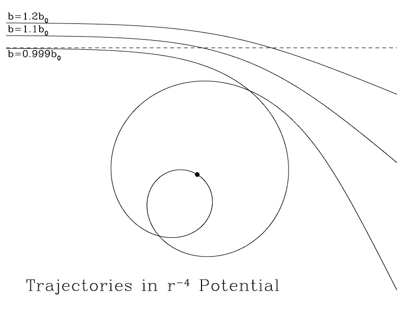
Three trajectories in a \(1/r^4\) potential. Attribution: Draine Figure 2.2
When \(b < b_0\), the charged particle can undergo an “orbiting” trajectory, which has cross section for interaction \(\pi b_0^2\). If you do the math, this unique cross section leads to a rate coefficient \(\langle \sigma v \rangle\) that is independent of temperature.
See Draine Table 2.1 for a list of Ion-Neutral scattering parameters. We’re talking about neutrals like H, He, \(\mathrm{H}_2\), and O, and ions like \(H^+, C^+, \mathrm{H}_2^+\).
Orbiting trajectories bring ion and neutral into close contact, and if there is an energetically allowed outcome
- collisional dexcitation
- exothermic charge exchange
- chemical exchange reaction and the reaction rate coefficients for these reactions become comparable to the orbiting rate coefficient.
Because the rate coefficients are independent of temperature (all others we’ve examined are dependent on temperature), exothermic ion-neutral reactions play a major role in chemistry of cool interstellar gas.
Electron-Neutral Collision Rates
Elastic scattering of electrons by neutrals. Can be important in very low ionization environments (e.g., protoplanetary disks). Primary collision partner is \(H_2\). Rates are determined experimentally.
Neutral-Neutral Collision Rates
Interactions between two neutral species
- at small separations is repulsive
- at larger separations is attractive (van der Waals) \(U(r) \propto r^{-6}\)
The fact that attractive interaction is very weak and the onset of repulsive interaction sufficiently rapid that we can treat the two partners as “hard spheres,” i.e., the cross-sectional area is really just the characteristic size of the atom or molecule (~1 Å). Think of throwing two basketballs at each other. They will only interact if \(b < R_1 + R_2\), i.e., if the balls would hit each other. No need to consider effective cross sectional area for charges. For temperatures less than 100 K, the rate coefficient for neutral-neutral scattering is more than 10x smaller than the rate coefficient for ion-neutral scattering.
Review
- Collisions are fundamental to ISM physics
- We’ve introduced a simple framework for understanding collisional rate coefficients for different types of interactions