Spontaneous Emission, Stimulated Emission, and Absorption
- Draine Ch. 6: Spontaneous Emission, Stimulated Emission, and Absorption
- Ryden and Pogge Ch. 2.1: Radiative Transfer
- Ryden and Pogge Ch. 2.2: Absorbers and Emitters
- Lecture notes on Radiative Transfer in Astrophysics by C.P. Dullemond.
- Radiative Processes by Rybicki and Lightman
General rules for absorption and emission of radiation by absorbers with quantized energy levels. Can be atoms, ions, molecules, dust grains, or anything that has (quantized) energy levels.
Absorption of photons
Some absorber is in a lower level, there is radiation present that has $$ h \nu = E_u - E_l $$ the absorber can absorb a photon and undergo an upward transition $$ X_l + h \nu \rightarrow X_u. $$
Rate of this reaction
There is some \(n(X_l)\). The rate per volume at which absorbers absorb photons (\(l \rightarrow u\)) is proportional to the density of photons of the appropriate energy and the number density of absorbers
$$ \underset{\mathrm{populate\;level}\;u}{\left ( \frac{\mathrm{d}n_u}{\mathrm{d}t} \right )_{l \rightarrow u}} = \underset{\mathrm{depopulate\;level}\;l}{- \left ( \frac{\mathrm{d}n_l}{\mathrm{d}t} \right)} $$
$$ = n_l B_{lu} u_\nu $$
\(u_\nu\) is the radiation energy density per unit frequency.
\(B_{lu}\) is a proportionality constant called the Einstein B coefficient for the transition \(l \rightarrow u\).
Emission of photons
Spontaneous emission
$$ X_u \rightarrow X_l + h \nu $$
Random process (independent of radiation field), and occurs with a probability per unit time \(A_{ul}\) called the Einstein A coefficient.
Stimulated emission
$$ X_u + h \nu \rightarrow X_l + 2 h \nu $$
Occurs if photons of identical
- frequency
- polarization
- direction are present in a radiation field.
Rate of emission
From state \(u \rightarrow l\)
$$ \left ( \frac{\mathrm{d}n_l}{\mathrm{d}t} \right) = - \left ( \frac{\mathrm{d}n_u}{\mathrm{d}t}\right) = n_u (A_{ul} + B_{ul} u_\nu) $$
\(B_{ul}\) is the Einstein B coefficient for the downward transition.
Einstein coefficients are not independent
$$ B_{ul} = \frac{c^3}{8 \pi h \nu^3} A_{ul} $$
$$ B_{lu} = \frac{g_u}{g_l} B_{ul} = \frac{g_u}{g_l} \frac{c^3}{8 \pi h \nu^3} A_{ul} $$
Strength of stimulated emission (\(B_{ul}\)) and absorption (\(B_{lu}\)) are both determined by \(A_{ul}\) (spontaneous emission) and the ratio of the degeneracies \(\frac{g_u}{g_l}\).
Radiation fields
(Review from Rybicki and Lightman, Ch 1)
\(I_\nu \) is the specific intensity of radiation, you can think of it as the energy carried along by an infinitesimal “bundle” of rays.
It has dimensions $$ \mathrm{ergs}\;\mathrm{s}^{-1}\;\mathrm{cm}^{-2}\;\mathrm{ster}^{-1}\;\mathrm{Hz}^{-1} $$ I like calling \(I_\nu\) the “specific intensity,” and that seems to be common usage in astronomy. In non-astronomy settings, this is called “spectral intensity.” If it is integrated over all frequency, it’s sometimes called the radiant intensity \(I\).
\(I_\nu \) can be a little mind-bending to think about… it can be a function of
- 3D space
- direction
- frequency
Intensity itself is not a vector quantity but it is a scalar field that is function of direction. Draine and Rybicki and Lightman write the angular direction vector as \(\Omega\) and the solid angle surrounding that vector as \(\mathrm{d}\Omega\).
If we have a defined reference frame, we would probably write \(\Omega\) as a vector in spherical coordinates and define the components along \(\hat{\phi}\) and \(\hat{\theta}\) and let \(\mathrm{d}\Omega = d\phi \sin \theta d\theta\).
\(B_\nu\) is exactly the same type of variable, we just use it instead of \(I_\nu\) when we’re referring to blackbody radiation, specifically of the form $$ B_\nu = \frac{2 h \nu^3}{c^2}\frac{1}{e^{h \nu / kT} - 1} $$ it also has units of $$ \mathrm{ergs}\;\mathrm{s}^{-1}\;\mathrm{cm}^{-2}\;\mathrm{ster}^{-1}\;\mathrm{Hz}^{-1} $$
Flux
Once you’ve defined \(I_\nu\), then it’s relatively easy to calculate quantities like energy density, flux, momentum, etc, as integrals of the specific intensity field.
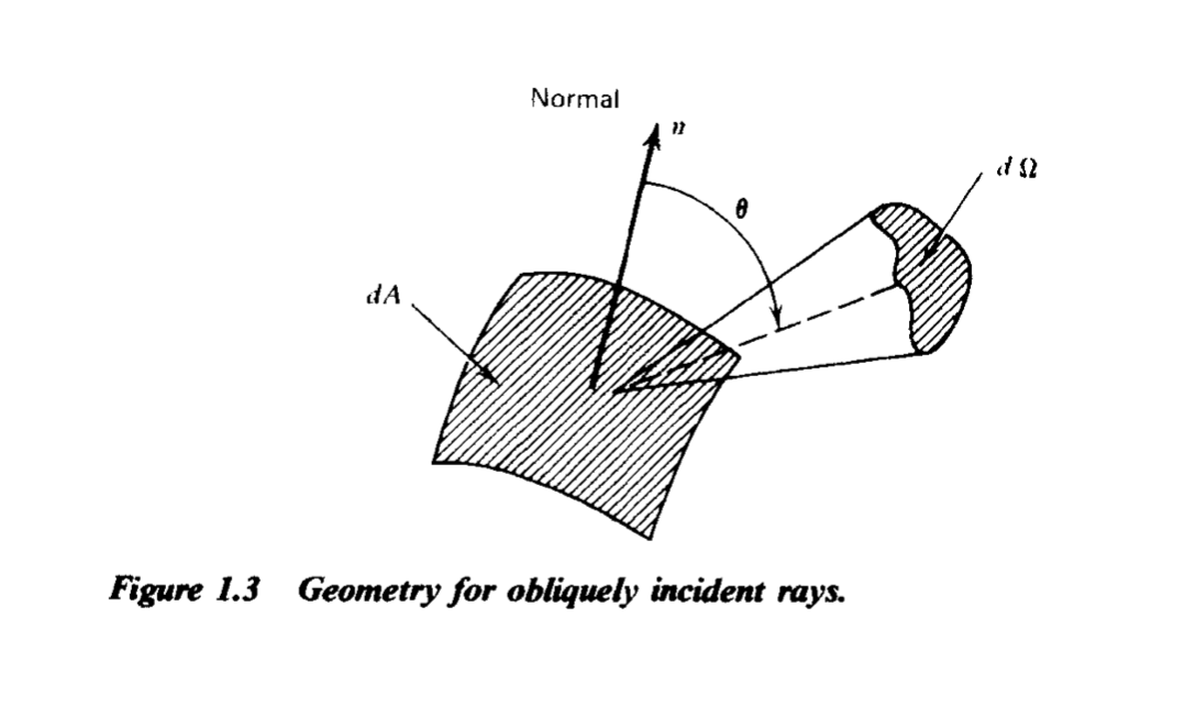
How to calculate flux from specific intensity. Credit: Rybicki and Lightman Ch. 1
$$ F_\nu = \int I_\nu \cos \theta d \Omega $$ (intensity passing through some differential area \(dA\), lowered by the effective angle).
\(F_\nu\) has units of $$ \mathrm{ergs}\;\mathrm{s}^{-1}\;\mathrm{cm}^{-2}\;\mathrm{Hz}^{-1} $$ (i.e., angular dependence has been integrated out). I like using the unit of Jansky, which is $$ 1\,\mathrm{Jy} = 10^{-23} \mathrm{ergs}\;\mathrm{s}^{-1}\;\mathrm{cm}^{-2}\;\mathrm{Hz}^{-1} $$
In astronomy settings, \(F_\nu\) is called the spectral flux density. In non-astronomy settings, this is called spectral irradiance. Sometimes you will see \(F_\lambda\), which has units $$ \mathrm{ergs}\;\mathrm{s}^{-1}\;\mathrm{cm}^{-2}\;\mathrm{cm}^{-1} $$ (or per Å, depending on your wavelength range).
Note that \(F_\nu\) and \(F_\lambda\) are flux densities or distribution function, which means that $$ F_\nu \ne F_\lambda $$ (their units are different)!
What is true is $$ F_\nu \mathrm{d}\nu = F_\lambda \mathrm{d}\lambda $$ because we’re comparing two quantities with units $$ \mathrm{ergs}\;\mathrm{s}^{-1}\;\mathrm{cm}^{-2} $$
You’ll sometimes also see a spectral energy distribution plotted $$ F_\nu \nu = F_\lambda \lambda $$ this comes about because $$ \nu = \frac{c}{\lambda} $$ $$ \frac{d \lambda}{d \nu} = -\frac{c}{\nu^2} = -\frac{\lambda}{\nu} $$ and the minus sign goes away because fluxes are defined per positive unit of frequency or wavelength.
I find the question of whether we’re referring to
- \(I_\nu\): specific intensity (Jy/ster)
- \(F_\nu\): spectral flux density (Jy)
- \(F\): Bolometric flux \(\mathrm{ergs}\;\mathrm{s}^{-1}\;\mathrm{cm}^{-2}\).
to be endlessly confusing in conversation, because it’s very common to colloquially use “flux” or “brightness” to mean a range of quantities, even though they have specific definitions in many settings. I find the clearest thing is to state the variable \(I_\nu\) or \(F_\nu\) (or \(F_\lambda\)) and the units.
Energy density and photon occupation number
The “mean” (directionally averaged) intensity is $$ J_\nu = \frac{1}{4 \pi} \int I_\nu d \Omega = \frac{1}{4\pi} \int I_\nu \sin \theta d \theta d\phi. $$ it has a different meaning than flux. In an isotropic radiation field, the net flux will be 0, whereas the mean intensity will have some positive value.
and the mean radiation density is $$ u_\nu = \frac{4 \pi}{c} J_\nu. $$ these quantities are not a function of direction, since we’ve averaged over it.
For a thermal, blackbody spectrum, we have $$ u_\nu = \frac{4 \pi}{c} B_\nu(T) $$
In equilibrium, the absorbers must have levels populated according to $$ \frac{n_u}{n_l} = \frac{g_u}{g_l}e^{(E_l - E_u)/kT} $$
The following doesn’t depend on thermal equilibrium
We can also write down the photon occupation number \(n_\gamma\), i.e., a dimensionless quantity tracking how many photons exist “per given solid angle”
$$ n_\gamma = \frac{c^2}{2 h \nu^3} I_\nu $$
which we can average over all directions to get $$ n_{\mathrm{bar},\gamma} = \frac{c^3}{8 \pi h \nu^3} u_\nu $$ (a truly dimensionless quantity).
These photon occupation numbers make it easy to rewrite the transition rates.
From \( u \rightarrow l\) $$ \left ( \frac{dn_l}{dt}\right)= n_u A_{ul} (1 + n_{\mathrm{bar},\gamma}) $$
Stimulated emission is not important when \( n_{\mathrm{bar},\gamma} \ll 1 \).
From \( l \rightarrow u\) $$ \left ( \frac{d n_u}{dt} \right ) = n_l \frac{g_u}{g_l} A_{ul} n_{\mathrm{bar},\gamma} $$
Absorption cross section
Because we’re talking about photons, instead of a velocity-dependent cross section, we will write a frequency-dependent cross section, \(\sigma(\nu)\). The velocity will be the speed of light \(c\).
Photon density [1/cm^3] per unit frequency $$ \frac{u_\nu}{h \nu} $$
Like in Ch 2, we would rate a rate as $$ n_A n_B \langle \sigma v \rangle $$ we’ll do the same thing with \(n_l\), \(\frac{u_\nu}{h \nu}\), and \(\sigma(\nu)\).
For the \(l \rightarrow u\) transition, $$ \left ( \frac{d n_u}{d t} \right ) = n_l \int d \nu \sigma_{lu}(\nu) c \frac{u_\nu}{h \nu}. $$
We can relate this back to the Einstein B coefficient for absorption to find $$ B_{lu} = \frac{c}{h \nu} \int d\nu \sigma_{lu}(\nu) $$ relate this back to the \(A_{ul}\) coefficient, $$ \int d_\nu \sigma_{lu}(\nu) = \frac{g_u}{g_l} \frac{c^2}{8 \pi \nu^2_{lu}} A_{ul}. $$ Then solve for \(\sigma_{lu}(\nu)\) $$ \sigma_{lu}(\nu) = \frac{g_u}{g_l} \frac{c^2}{8 \pi \nu^2_{lu}}A_{ul} \phi_\nu $$ where \(\phi_\nu\) is a normalized line profile $$ \int \phi_\nu d \nu = 1. $$
Oscillator strength
You can also write these relationships with something called the oscillator strength, \(f_{lu}\). $$ A_{ul} = \frac{8 \pi^2 e^2 \nu_{lu}^2}{m_e c^3} \frac{g_l}{g_u} f_{lu} $$
Intrinsic line profile
A Lorentzian is a good description of the intrinsic line profile (need quantum mechanical calculation to get it exact).
$$ \phi(\nu) = \frac{4 \gamma_{ul}}{16 \pi^2(\nu - \nu_{ul})^2 + \gamma_{ul}^2} $$
The intrinsic width of the absorption line reflects the uncertainty in the energies of levels \(l,u\) due to the finite lifetimes against transitions to other levels.
Intrinsic widths of lines \(\propto h \nu\), which means x-ray transitions can have considerably larger line widths than radio transitions (assuming the medium is stationary).
We’ll talk more about absorption line profiles, Doppler broadening, Voigt profiles, etc… in a few lectures.