Introduction to Radio Astronomy and ALMA
Suggested reading: ALMA Primer
Resources:
- Essential Radio Astronomy by James Condon and Scott Ransom (HTML book)
- Interferometry and Synthesis in Radio Astronomy, 3rd Edition by Thompson, Moran, and Swenson. Electronically available from PSU library.
- Tools of Radio Astronomy by Wilson and Hüttemeister. Also electronically available from PSU library.
- NRAO Summer School Lectures and Slides
- The Fourier Transform and its Applications by R. Bracewell
Disclaimer: Radio astronomy (including radio interferometry) is a vast subject area worthy of several full length courses. I encourage you to check out the resources above to survey the many topical areas that we won’t be able to cover in this lecture.
Goal: provide enough of an introduction to radio astronomy, radio interferometry, and the concepts relevant to ALMA, such that you see some of the connections possible with our mock TAC and scientific justification later in the course.
Atmospheric Windows
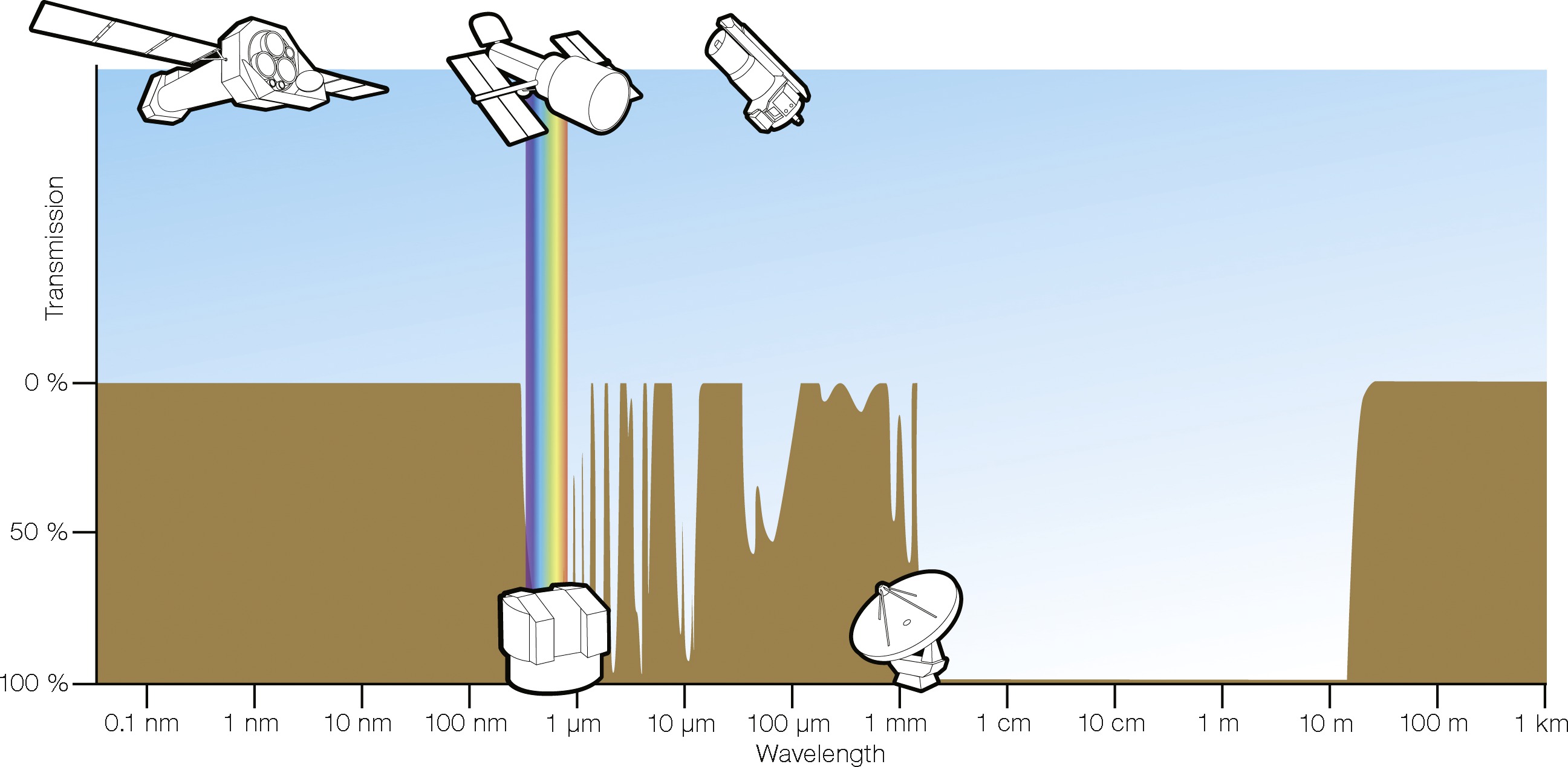
Atmospheric windows for astronomy. Credit: ESA/Hubble (F. Granato) and Essential Radio Astronomy.
By comparison to optical windows, the radio region of the spectrum is downright transparent. Only towards very high radio/microwave frequencies (wavelengths about 1 mm), does the atmospheric transmission start to decline.
The same $$ \theta \approx \frac{\lambda}{D} $$ applies for radio antennas. Take a \(\lambda = 1\;\mathrm{cm}\) observation, for example. Compared to an optical \(\lambda = 500\;\mathrm{nm}\) telescope the same size, the resolution will be a factor of $$ \frac{1\;\mathrm{cm}}{500\;\mathrm{nm}} = 20,000 $$ worse. Yikes!
Radio astronomers are constantly trying to find ways to increase angular (spatial) resolution.
- One way is to build bigger telescopes, such as the Green Bank Telescope (100m diameter)
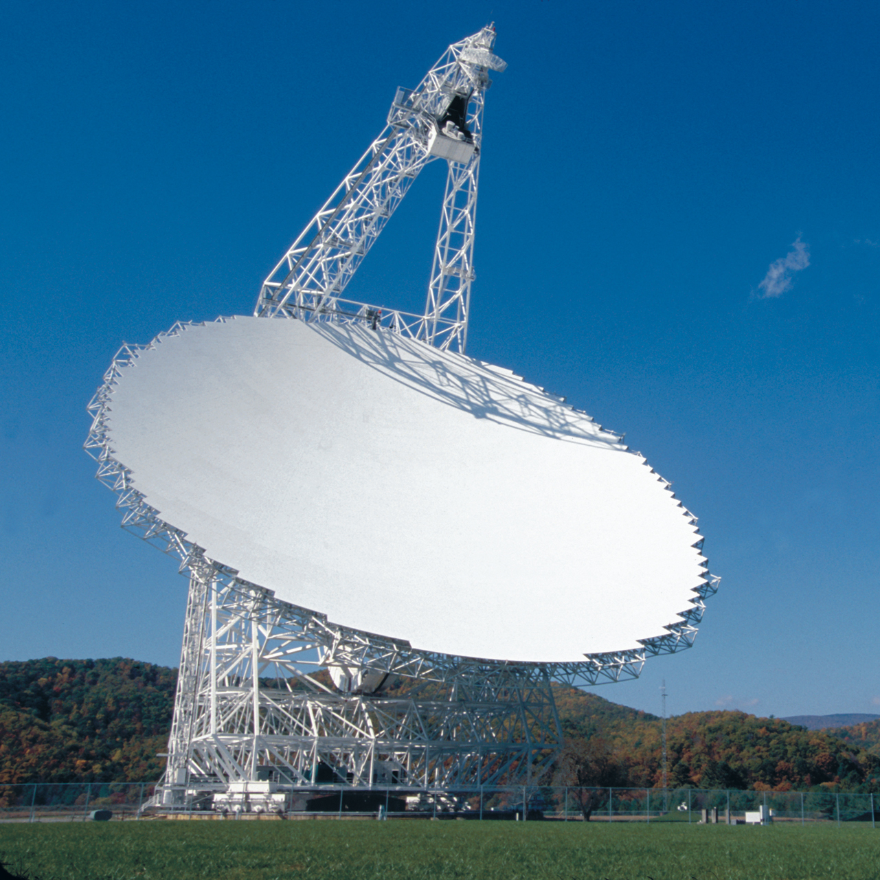
The Green Bank Telescope (100m diameter) operates at radio wavelegths. Credit: NRAO/AUI/NSF
- Another way is to work at higher frequencies (shorter wavelengths), e.g. sub-mm radio astronomy (IRAM 30m telescope)
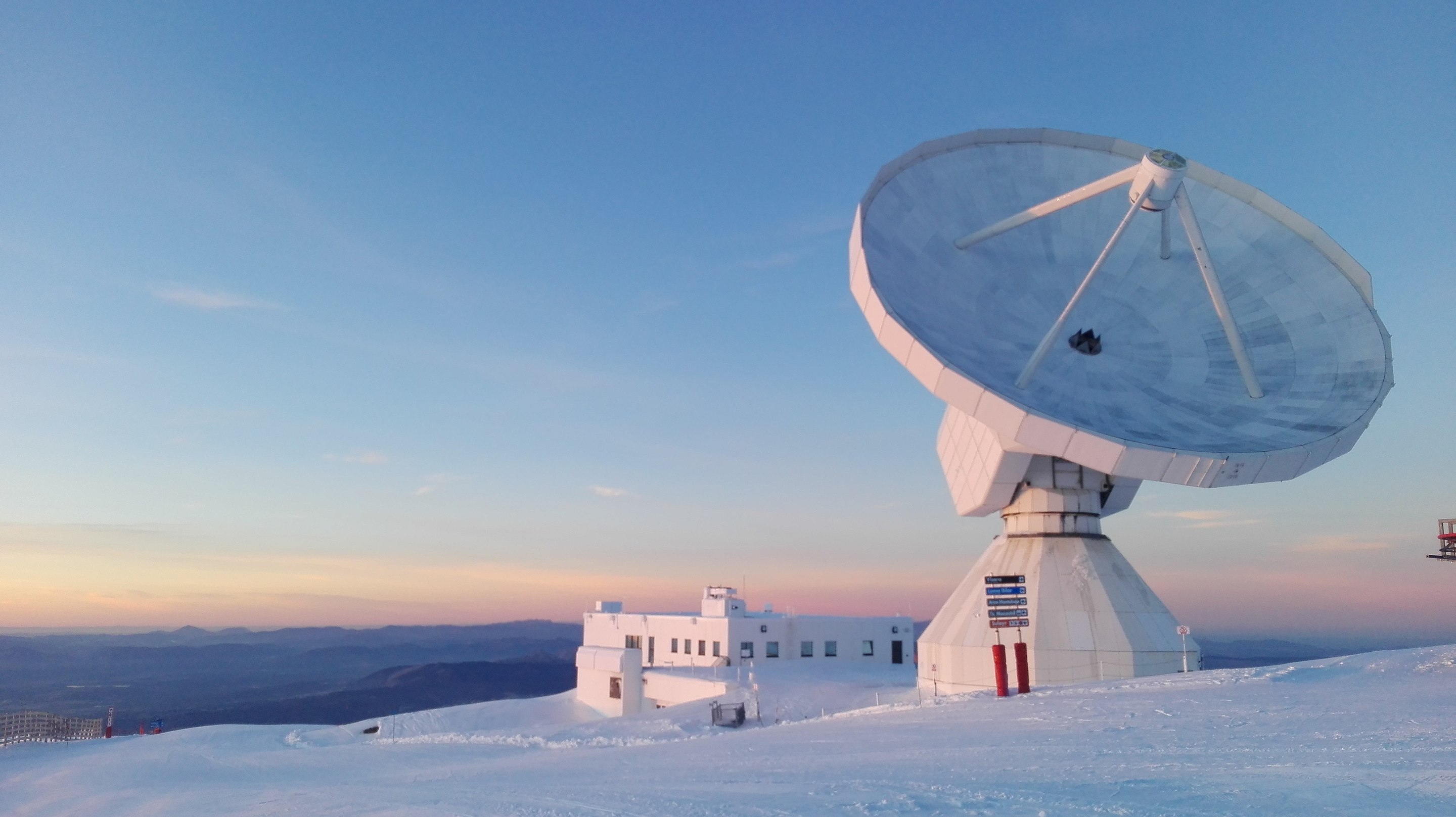
The IRAM 30m diameter telescope, which operates at sub-mm wavelengths. Credit: Wikipedia/IRAM-gre
- A final way is to use interferometry, sometimes also at sub-mm wavelengths (ALMA)
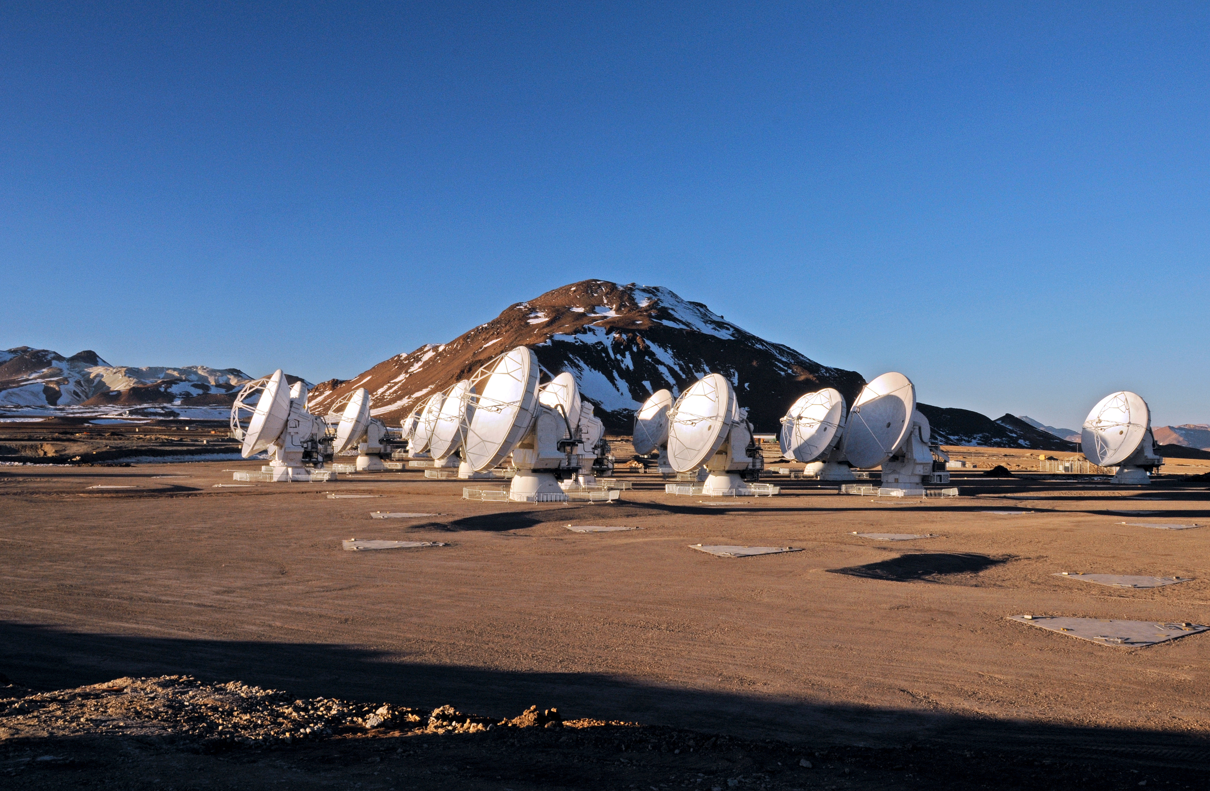
The Atacama Large (Sub)millimeter Array, an interferometric array of 66 antennas operating at sub-millimeter wavelengths. The largest antennas in the array are only 12m in diameter, yet through interferometry, the array is able to obtain far higher spatial resolution than the largest single-dish antennas. Credit: NRAO/ESO/NAOJ/JAO
It’s easier to build larger telescopes at longer wavelengths because the tolerances required for the reflecting surface are less strict than at optical wavelengths. Though typically one must keep surface tolerances to within $$ \sigma = \frac{\lambda_\mathrm{min}}{16}, $$ otherwise the efficiency of the antenna starts to decline substantially. For the 100 m diameter GBT operating at it’s highest frequency (100 GHz) or 3 mm, this translates to \(200\;\mu\mathrm{m}\), which is the thickness of two sheets of paper! That’s quite an engineering challenge, and is the reason why large, steerable dishes are difficult to build.
Keeping telescopes fixed is one way to build a little bit bigger, such as FAST, which is a five hundred meter diameter fixed telescope in China. See also Arecibo, which unfortunately collapsed in December 2020. Eventually, though, the materials/engineering cost to building large single dish telescopes becomes prohibitive.
Single dish observations
The “beam” or power pattern as a function of direction, of a receiving antenna can be calculated using the reciprocity theorems for transmitting and receiving antennas. We don’t have time to cover it in this lecture, but the end result is that the far field electric field pattern \(f(l)\) is the Fourier transform of the electric field illuminating the aperture of the telescope \(g(u)\).
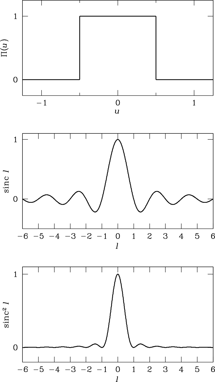
A schematic illustration of (top): Uniformly illuminated aperture (middle): The electric field pattern of the antenna, as a function of direction (bottom): The power pattern of the antenna, as a function of direction. Credit: Essential Radio Astronomy
For large apertures, the nulls at \( l = \pm 1, 2, \ldots\) appear at the angles \(\theta \approx \lambda/D, 2 \lambda/D, \ldots\). In two dimensions, for a circular aperture, this is an Airy pattern.
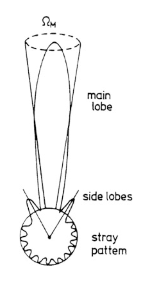
A beam power pattern plotten in polar coordinates, demonstrating that the antenna can pick up power from sidelobes at range of angles. Credit: Tools of Radio Astronomy.
This is an idealized representation, but is still helpful. The beam can pick up power through sidelobes at a range of angles. Directional antennas help concentrate power in the main beam, but antennas with secondary stages (and thus supports, like most telescopes) create opportunities for ground radiation to reflect into the receiver. The relationship between the aperture and the electric
You can think of single-dish telescopes (unless they have a sophisticated, multi-pixel receiver) essentially as single-pixel devices. So to make a map of the sky, you would need to raster scan the telescope across the region of interest, reading out antenna temperature as a function of RA, Dec. To make a good (i.e., scientifically accurate) map, you should focus on Nyquist sampling the sky to a uniform sensitivity, usually through a hexagonal pattern of dithering. More advanced instruments may have an array of “feeds” in a focal plane (mirroring a set of “pixels”), but this is still a small number of pixels compared to a typical CCD (e.g., 25 or 36).
Temperatures, redux
In an earlier lecture, we gave definitions of “brightness temperature” and “antenna temperature” following Draine
- brightness temperature: the temperature corresponding to the specific intensity if we used the full form of the Planck formula
- antenna temperature: the temperature corresponding to the specific intensity if we were in the Rayleigh-Jeans domain. Added benefit that specific intensity is linearly related to antenna temperature and makes it easy to substitute one for the other. $$ T_A(\nu) = \frac{c^2}{2 k \nu^2} I_\nu $$
These definitions are still true, but also somewhat idealized, as we’ll cover in a second.
In the field of radio astronomy, be aware that one frequently combines temperatures in other interesting ways. One can express random noise power in terms of an effective temperature $$ P = k T \Delta \nu $$ where \(\Delta \nu\) is the bandwidth of the observation. Here the power is equal to the noise power delivered to a matched load by a resistor at physical temperature \(T\). By matched load, we mean we connect a resistor to the input terminals of a linear amplifier. The fact that this resistor has some temperature (i.e., we haven’t cooled it to absolute zero…) means that the thermal motion of the electrons will produce a random, variable current \(i(t)\) input to the amplifier. The mean value of this current is zero, but the root mean squared value is non-zero, and this represents a non-zero power. I.e., you can draw (some) power from a resistor at room temperature, purely from thermal motions. The situation is not dissimilar to the random walk of a particle in Brownian motion. For more details, see Tools of Radio Astronomy, Chapter 1.8.
- Antenna temperature \(T_A\) the component of the power received by the antenna from cosmic sources. It has the same interpretation as before (though we’ll talk about beam dilution in a second).
- Receiver temperature \(T_R\) the component of the power from internal noise of the receiver components themselves, ground radiation, atmospheric emission, etc…
- System temperature \(T_S = T_A + T_R\) is the sum of receiver temperature and antenna temperature. It’s the one power number coming out of the backend of your telescope. It’s up to you to calibrate \(T_R\) accurately enough to measure \(T_A\).
In any observation, you will have your cosmic signal of interest and several contributions of noise (see Essential Radio Astronomy, Ch. 3.6.1) $$ T_S=T_\mathrm{cmb}+T_\mathrm{rsb}+T_A + [1−\exp(−\tau_A)] T_\mathrm{atm}+T_\mathrm{spill}+T_r+ \ldots $$ such as the CMB, other galactic background sources, the atmosphere, spillover radiation from the ground, the temperature of the radiometer itself (hopefully cryogenically cooled), etc.
In the limit that \(T_A \ll T_S\) (most astronomy situations, unfortunately!), we have $$ S/N \approx C \frac{T_A}{T_S} \sqrt{\Delta \nu \Delta t} $$ where \(C\) is a constant of proportionality greater than or equal to 1, and \(\Delta t\) is the integration time. If we let \(\Delta \nu \approx 1\;\mathrm{GHz}\) and \(\Delta t \approx 1\;\mathrm{h}\), then we can get \(\sqrt{\Delta \nu \Delta t} \approx 10^6\), allowing us to detect a signal which is less than \(10^{-6}\) the system noise. A great illustration of this capability is the COBE satellite that studied CMB anisotropies with brightness temperatures \(< 10^{-7}\) that of the system temperature. To achieve these contrasts, however, it’s important to keep systematics under control, otherwise the S/N scaling won’t hold!
Beam dilution
In previous lectures, we’ve been talking about specific intensity \(I_\nu(\Omega)\) as a “known” quantity of direction (e.g., R.A., Dec.) and used antenna temperature \(T_A\) as a linear proxy for its specification. For the following discussion, we’re going to move into the realm of observations, and discuss the ways \(T_A\) can be an unfaithful proxy for the “true” specific intensity distribution or brightness temperature. we’ll use the symbol \(T_b(\Omega)\) to denote the “true” brightness/antenna temperature, assuming we’re in the Rayleigh-Jeans limit, and redefine \(T_A\) to mean the response of the telescope to the cosmic radiation.
When we’re doing observations, we don’t always have access to the highest resolution version of \(T_b(\Omega)\), but rather we have access to a quantity which is the true \(T_b(\Omega)\) convolved with the beam of the telescope, which is the implication of \(T_A\) for this discussion.
large (fully resolved) source
[Draw a smooth cloud with the beam overlaid as a small circle].
In the limit that we are observing a source that subtends a solid angle much larger than the beam of the antenna, $$ \Omega_S > \Omega_A $$ the convolution of the beam doesn’t matter, we’re still sensing approximately the same \(T_b(\Omega)\) such that $$ T_A(\Omega) \approx T_b(\Omega). $$ If the source is in LTE, then we also have that \(T_A \approx T\).
small (unresolved) source
[Draw a beam with a smaller source in the center]
If the source is more compact than the antenna beam, $$ \Omega_S < \Omega_A, $$ then the measured antenna temperature is basically the “true” intensity averaged over the area of the main beam. This lowers the measured antenna temperature by a factor $$ \frac{T_A}{T_b} = \frac{\Omega_S}{\Omega_A} $$ where the ratio \(\frac{\Omega_S}{\Omega_A}\) is called the beam filling factor.
For example, you could have a compact source with \(T_b = 10^4\) K, but if it only fills 1% of the beam solid angle then you would measure an antenna temperature of 100 K. If you took your observations at face-value (and assumed LTE), then you would incorrectly conclude that the source is 100x cooler than it actually is.
Beam dilution also applies to observations of sources that have structure on spatial scales below the observable limit, which, to be honest, is going to be most astrophysical sources of interest. For example, consider a gas filament in a star-forming region.
[Draw an approximation of a gas filament]
Radio-bright, spatially concentrated regions will be “smeared out” by the beam. If you wanted to use antenna temperature (and assume LTE) to estimate the physical conditions of the gas filament, you do so at the peril of measuring incorrect temperatures. The unfortunate reality here is that, without higher resolution images to guide you (which sometimes exist at optical or infrared wavelengths), it’s quite difficult to estimate how badly your measurements are affected by beam dilution.
point source
In the case of an unresolved point source with known flux \(F_\nu\), it’s not that helpful to talk about brightness temperatures if we can’t also estimate the solid angle that the source subtends \(\Omega_S\), since it is required to relate flux to specific intensity (or brightness temperature). [Sometimes we can estimate \(\Omega_S\) from theoretical arguments, even if the source is so small as to still be unresolvable, in which case we’d still use the above calculations.]
For point sources, it’s easier to talk about antenna temperature using $$ T_A = \frac{P_\nu}{k} = \frac{A_e F_\nu}{2 k} $$ where \(A_e\) is the effective collecting area of the telescope. This gives us the strange but sometimes convenient relationship of talking about a telescope’s sensitivity to a point source using “kelvins per jansky,” which is proportional to its collecting area.
For more useful single-dish guidance, see these notes by James Jackson, or Ch 3.1.6 of Essential Radio Astronomy.
Interferometers
Two-element interferometer
We’ll focus our discussion around the two-element interferometer, since even arrays of antennas (like ALMA) can be understood by breaking them down (conceptually) into this fundamental unit.
Consider two antennas separated by some distance \(b\) simultaneously observing a source. Unless the source is directly overhead, the radiation from the source will arrive at the antennas at slightly different times, corresponding to a geometric time delay \(\tau_g\). The voltage streams from these two antennas \(V_1\) and \(V_2\) are then correlated (multiplied together and then averaged) to form the output stream \(R\).
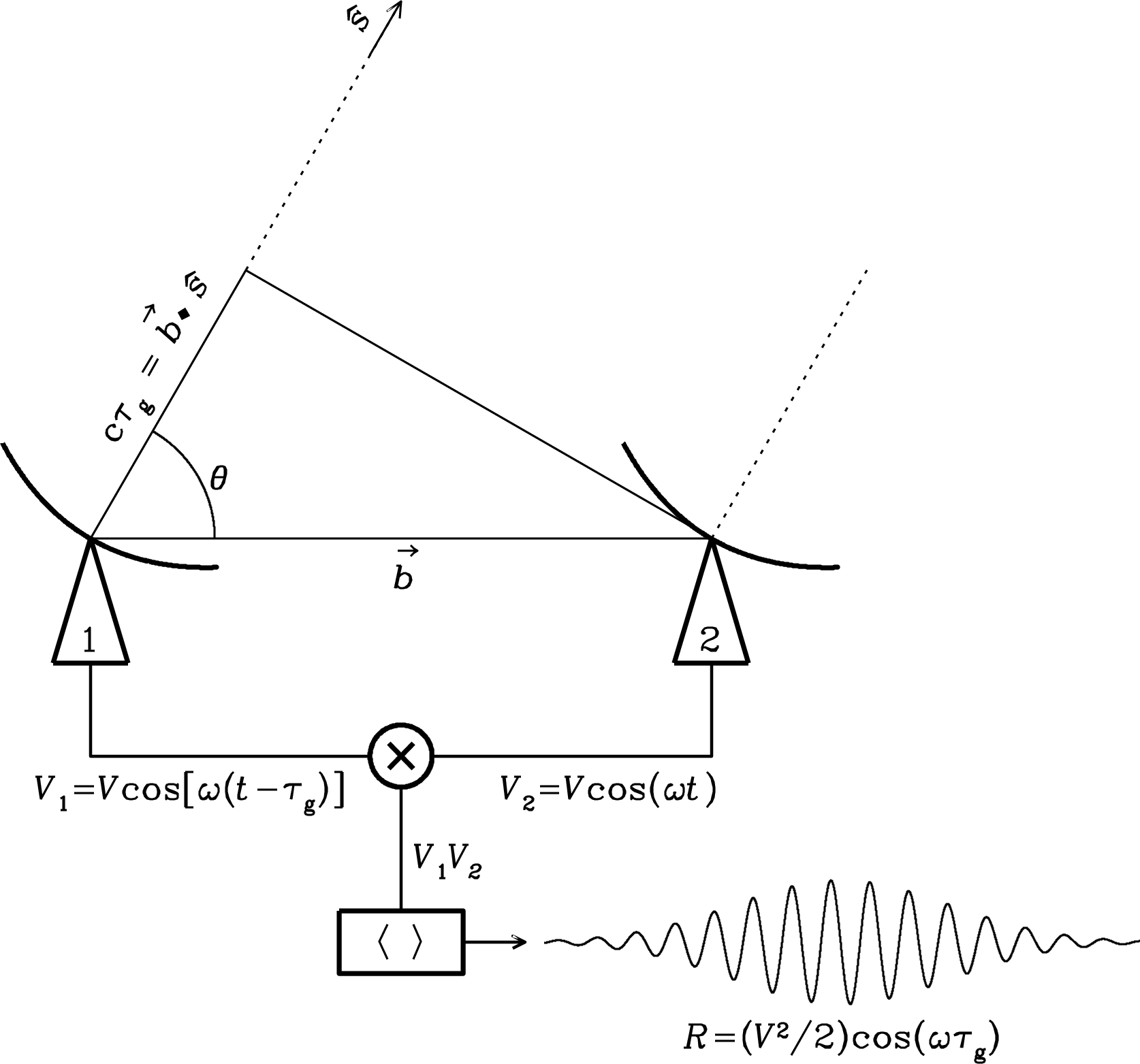
A schematic of a two-element interferometer. Credit: Essential Radio Astronomy
For now, we’ll call this a cosine correlator because of the cosine dependence of the correlation stream.
The fringe pattern in the lower right of this figure is what you would get if you kept the antennas stationary and let a point source drift across the field of view. The broad envelope is the attenuation from the primary beam response of the antennas as the source enters and then leaves the field of view. The fringe frequency depends on the observing frequency and the baseline separating the antennas.
Interestingly, the time averaged response of a multiplying interferometer has a mean of 0. This has the consequence that uncorrelated noise power from very extended sources (such as the CMB) will average to 0, therefore, the interferometer is not sensitive to radiation on those large spatial scales. This is called spatial filtering.
Multiple antennas
With multiple pairs of antennas, we can build up an improved point source response, because the fringe patterns of the individual two-element interferometers add up.
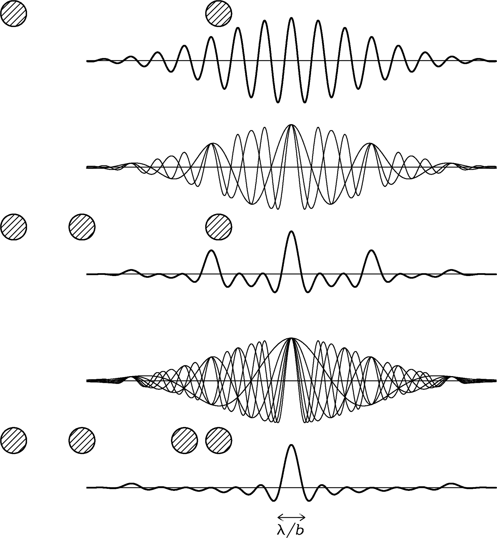
How the fringe patterns of the individual two-element interferometers in an array build up to create a beam. Each shaded circle represents an antenna spaced out along a 1D line. Credit: Essential Radio Astronomy.
In the limit of many antennas, the beam usually looks like something centralized, approximately Gaussian, but usually containing many sidelobes (hence, why radio astronomers call this a “dirty beam”).
The resolution of the beam is on the order of \(\lambda/b\), where \(b\) is the projected baseline of the longest antenna pair. Note that this resolution strongly depends on the relative number of baselines at long/short separations. It won’t suffice to just have a single long-baseline pair of antennas if most other antenna pairs are at much shorter baselines.
Complex correlators
Now let’s move beyond a discussion of point sources and consider what we’ll call a “slightly extended source,” something that is larger than the dirty beam but smaller than the primary beam of each telescope.
Instantaneous field of view of an interferometer is the same as the primary beam of each telescope, treated as a single dish (see previous section). Each single dish antenna is still seeing the same thing as before, it’s just that we have a correlator backend that’s doing things with the signals, allowing us to place many synthesized beams within the area of the primary beam.
The cosine correlator we discussed has some limitations, namely that the quantity $$ R_c = \int I(\hat{s}) \cos(2 \pi \vec{b} \cdot \hat{s}/\lambda) d\Omega $$ term is only sensitive to the even (symmetric) component of a source.
[Draw cosine curve centered around \(\vec{b} \cdot \hat{s} = 0 \), show that there is ambiguity in the response.]
We can decompose any function into a sum of its even and odd (antisymmetric) parts. To capture the odd parts of the source, we need a different kind of correlation, $$ R_s = \int I(\hat{s}) \sin(2 \pi \vec{b} \cdot \hat{s}/\lambda) d\Omega $$ which can be obtained by inserting a \(\pi/2 = 90^\circ\) phase delay in the output of one antenna.
When we combine cosine and sine correlators (in hardware, this is all the same system), we have what is called a complex correlator. It is usually more convenient to treat the cosine and sine components simultaneously using Euler’s formula and we have $$ \mathcal{V} = R_c - i R_s $$ or $$ \mathcal{V} = \int I(\hat{s}) \exp(- i 2 \pi \vec{b} \cdot \hat{s}/\lambda) d\Omega. $$ The quantity \(\mathcal{V}\) is called the visibility and it is a complex number. It is the fundamental data product from an interferometer, and, like all data, it is usually measured with some noise. For more on this, see the MPoL notes on likelihood functions.
Coordinates
The equation we’ve just derived is fairly general, but let’s expand this a bit to the astronomical coordinate systems we’re more used to.
Rather than referring to the source brightness distribution with \(I_\nu(\hat{s})\), usually we’ll refer to some phase center. [Typically this is the direction the antennas are pointed (i.e., center of primary beam), but doesn’t need to be and can be changed after the fact in software.]
We can define the direction cosines in a tangent plane, such that we have \(l = \sin(\Delta \alpha \cos \delta)\) and \(m = \sin(\Delta \delta)\), where \(\alpha\) and \(\delta\) are R.A. and Dec., respectively.
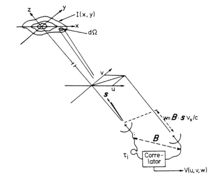
The relationship between baseline orientation, source position, and direction cosines \(x = l\) and \(y = m\). Credit: Tools of Radio Astronomy from Thompson 1982.
We can rewrite the projected baseline in terms of its east-west \(u\) and north-south \(v\) components, where
$$ u = \left [ \frac{\vec{b} \cdot \hat{s}}{\lambda} \right ]_\mathrm{east-west} $$
and
$$ v = \left [ \frac{\vec{b} \cdot \hat{s}}{\lambda} \right ]_\mathrm{north-south}. $$
So we have that the image domain coordinates \(l, m\) have corresponding Fourier plane coordinates \(u, v\), called spatial frequencies.
And the relationship between source brightness distribution and the visibility function is given by $$ \mathcal{V}(u,v) = \int \int I(l,m) \exp \{ - 2 \pi i (ul + vm)\} dl dm. $$ This is a two-dimensional Fourier transform.
It turns out that the measured spatial frequencies correspond directly to the projected baseline vector lengths, if the baseline is measured in multiples of the observing frequency.
Longer baselines measure higher spatial frequencies, which correspond to finer-scale image plane features.
Fourier Transform pairs
Here are some examples of Fourier transform pairs, where the left column represents the sky-plane intensity distribution \(I(l,m)\) and the right column represents the amplitude of the visibility function, \(|\mathcal{V}|^2\). (Remember, the visibility is a complex quantity, and also has a phase. Alternatively, it can be expressed in terms of its real and imaginary components.)
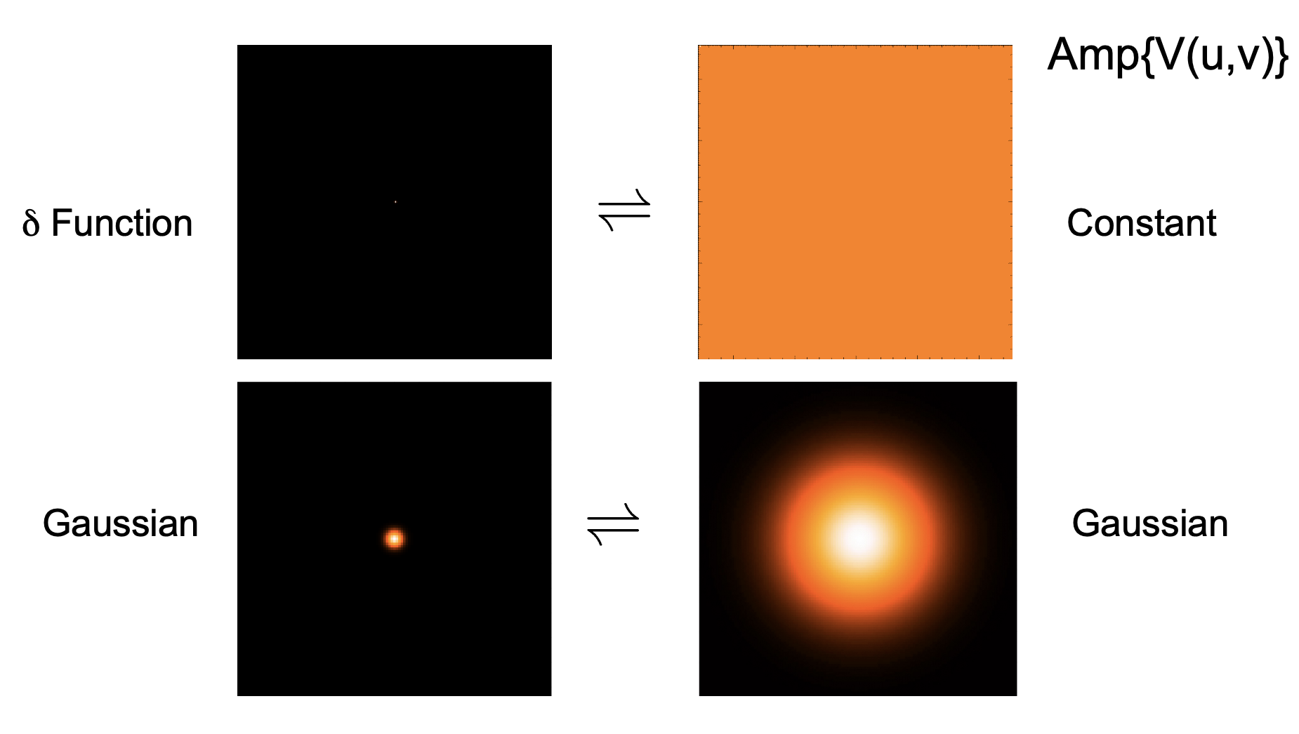
Narrower features in one domain will result in broader features in the other. Credit: David Wilner
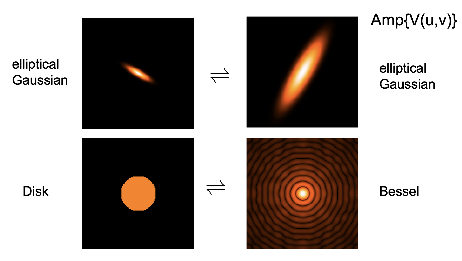
Sharp edges will result in power at high spatial frequencies. Credit: David Wilner
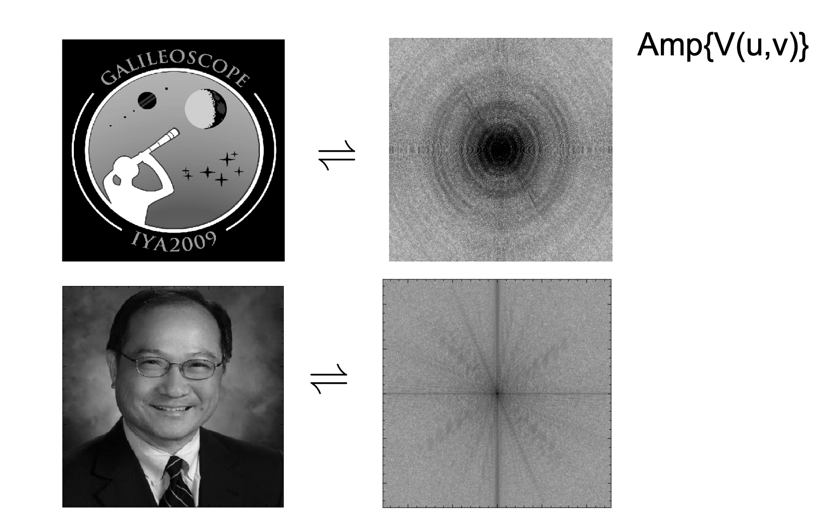
A real image (such as this picture of former NRAO director Fred Lo) has complicated structure on many scales. In general, a ’natural’ image will typically have more power at lower spatial frequencies than higher spatial frequencies. An example of a non-natural image is one containing text or artifical borders (lots of sharp lines), like the Galileoscope logo. Credit: David Wilner
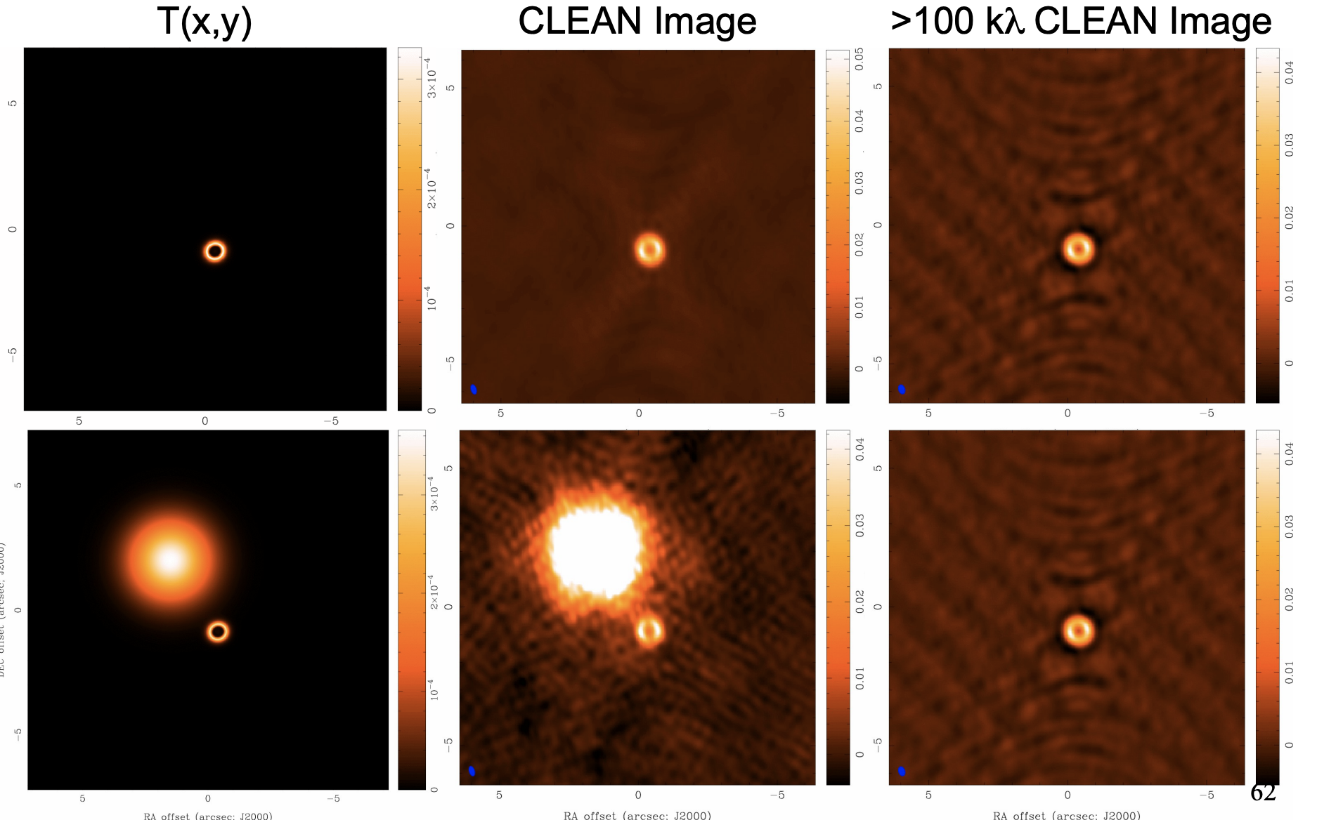
A demonstration of how an interferometer with an insufficient number of short baselines (right column) is insensitive to large-scale emission that is actually there (left column). This effect is especially important for studies of the ISM, where there can be diffuse emission from molecular clouds next to protoplanetary disks. Credit: David Wilner
Aperture synthesis
Because the earth rotates, the projected baseline to a source also changes throughout an observation. This can be used to great advantage to sample different spatial frequencies than were otherwise possible in a “snapshot” observation. The following is a video showing how UV coverage for the MAPS large program is built up over a series of eight 1-hour long observations, spaced out over a single year, and the corresponding “dirty beam” that results.
Making images from visibilities
How do go from the interferometric data samples of the visibility function to images? This is a complicated question.
We sampled the visibility function $$ \mathcal{V}(u,v) = \int \int I(l,m) \exp \{ - 2 \pi i (ul + vm)\} dl dm. $$ at a bunch of \(u,v\) points corresponding to the projected baselines of the array. There are many \(u,v\) points that we didn’t sample, and so it’s not possible to carry out the inverse Fourier transform completely accurately, with data alone.
What can we do?
- One approach is to not make images, and instead forward-model your data using a parametric model, like you might fit a line to a bunch of points. These are complex numbers, but the same principle applies. This has the benefit that you can do Bayesian inference on the parameters of the model (e.g., a Gaussian with some width at some location, etc…) but the drawback that you need to specify said model. For more information, see the discussion of model-fitting section of the MPoL documentation.
- Another is to fearlessly charge on and just take the direct inverse Fourier transform of the samples. This generates an image called the “dirty image,” because it retains the features of the dirty beam. The assumption here is that the unsampled spatial frequencies carry zero power (not a great assumption, in general), and their visibility values are set to zero. This means that the dirty image is highly sensitive to the array configuration, not something we want! The following movie shows the dirty image that results from choosing a different 75% of the dataset in a round robin fashion for each frame. There is no noise—each visibility is sampled perfectly.
There are several algorithms one can employ to try to recover the “true” sky brightness from the dirty image.
- CLEAN: iterative image-plane deconvolution. Build up a “CLEAN Model” using point sources, restore it with a “CLEAN beam,” which is typically a Gaussian.
- Regularized Maximum Likelihood (RML) imaging: forward-modeling of the visibilities (e.g., MPoL). Need to specify prior distributions in addition to the aforementioned visibility likelihood.
Science capacities of ALMA
In the remaining time, we’ll discuss the science capabilities of ALMA. A great resource for these materials is the