Introduction and Course Overview
References and Resources for this lecture
Full reference information can always be found in the syllabus, under “References Materials.”
- Essential Radio Astronomy Ch 1: emission mechanisms, relevant astrophysical objects
- Tools of Radio Astronomy: radio windows, units, flux densities
- Interferometry and Synthesis in Radio Astronomy: single-dish observations, units, flux densities
Course Overview
Welcome to Astro 589, a graduate seminar on radio astronomy and interferometric imaging!
- Syllabus overview regarding format, HW assignments, group project including proposal dates and presentation dates
Astrophysics at radio wavelengths
Emission mechanisms
- Radio synchrotron (continuum), non-thermal emission from relativistic electrons in magnetic fields
- Bremsstrahlung (a.k.a. free-free) emission (continuum), thermal emission from ionized gas (H II regions)
- Thermal emission from cold (< 100 K) media, like dust (continuum)
- Atomic hyperfine splitting (“21-cm” line corresponding to neutral hydrogen)
- Molecular emission lines, primarily from rotational transitions (e.g., CO \(J=2-1\))
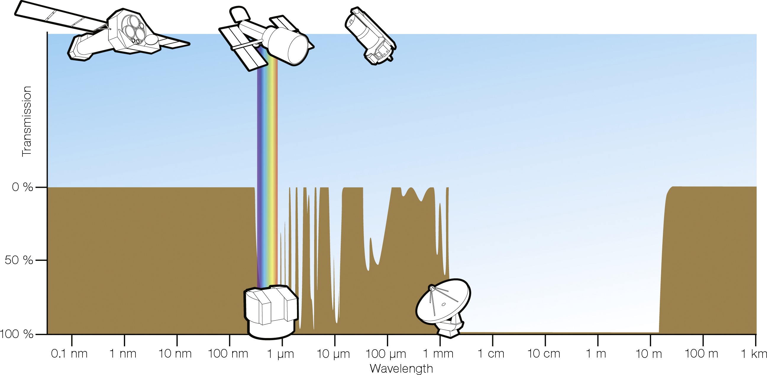
Atmospheric windows for astronomy. Credit: ESA/Hubble (F. Granato) and Essential Radio Astronomy.
The earth’s atmosphere is very transparent in the radio region of the electromagnetic spectrum, especially compared to optical windows. Only towards the microwave region (wavelengths around 1 mm), does the atmospheric transmission start to decline.
Astrophysical objects
In truth, almost everything these days!
- quasars
- gamma ray burst (GRB) afterglows
- fast radio bursts (FRBs)
- pulsars
- supernovae remnants
- cosmic microwave background (CMB)
- galaxies, including molecules at high redshift sources
- dust/interstellar medium
- the Sun
- planets (e.g., Jupiter, Uranus)
- protoplanetary disks
- molecular clouds (molecular emission)
- black hole accretion disks (EHT)
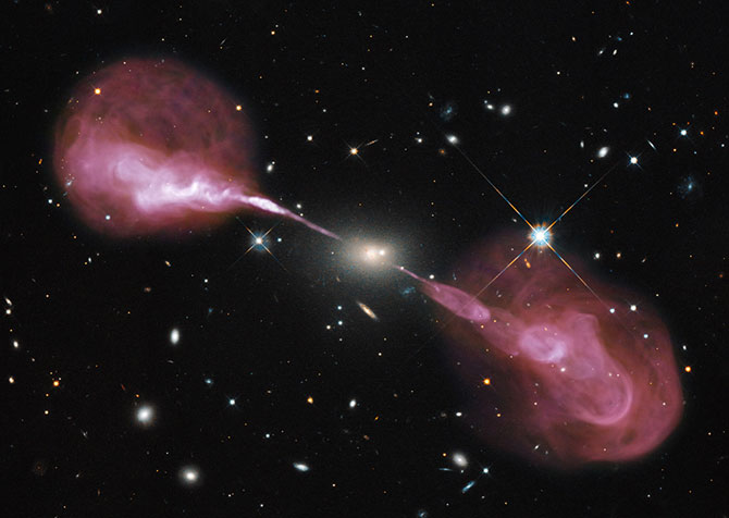
Radio jets from the elliptical galaxy Hercules A (overlaid with an optical image from Hubble). Karl Jansky VLA. Credit: NASA, ESA, S. Baum and C. O’Dea (RIT), R. Perley and W. Cotton (NRAO/AUI/NSF), and the Hubble Heritage Team (STScI/AURA).
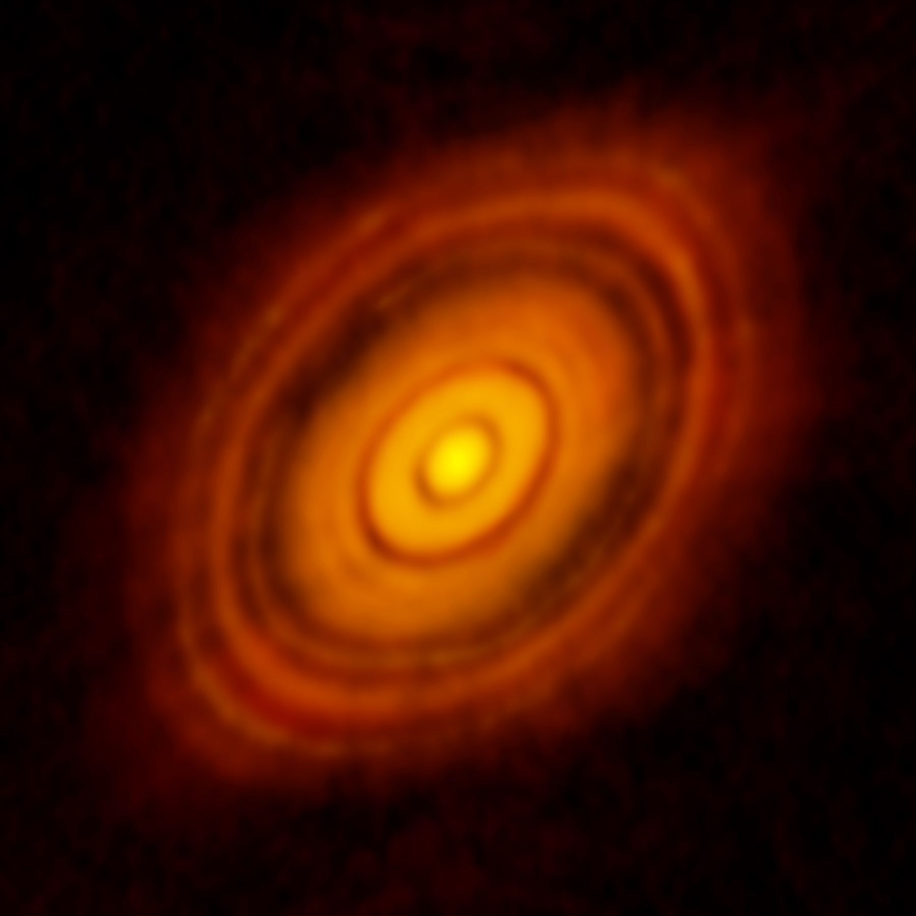
The protoplanetary disk around HL Tau, imaged using the Atacama Large Millimeter Array. Credit: ALMA(ESO/NAOJ/NRAO); C. Brogan, B. Saxton (NRAO/AUI/NSF)
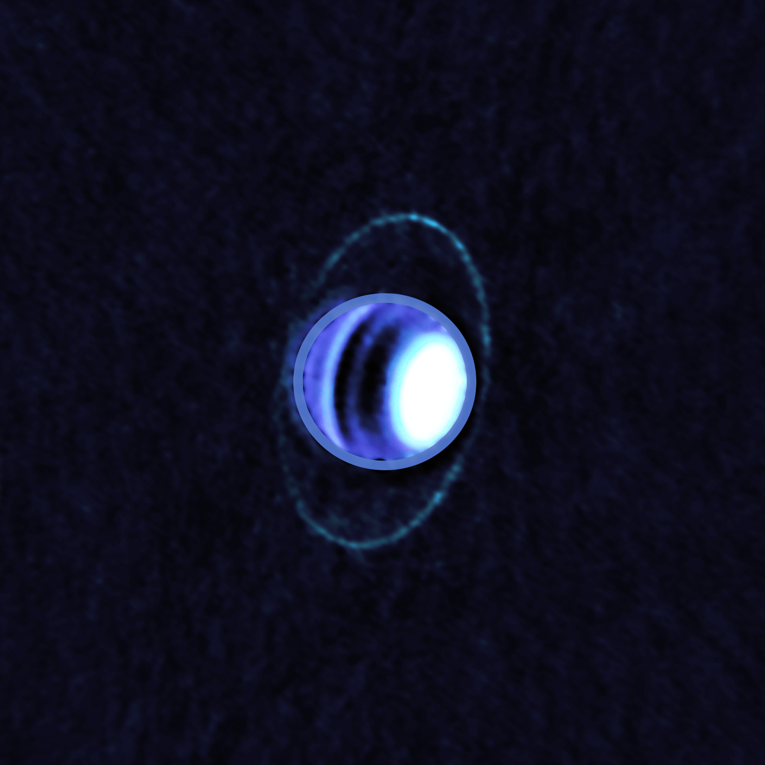
The rings of Uranus seen by ALMA (thermal emission from 77 K material). Credit: ALMA (ESO/NAOJ/NRAO); E. Molter and I. de Pater.
Single-dish radio telescopes
In this section, we’ll cover existing single-dish radio telescopes and refresh our memory of basic telescope performance.
The same $$ \theta \approx \frac{\lambda}{D} $$ applies for radio antennas. Take a \(\lambda = 1\;\mathrm{cm}\) observation, for example. Compared to an optical \(\lambda = 500\;\mathrm{nm}\) telescope the same size, the resolution will be a factor of $$ \frac{1\;\mathrm{cm}}{500\;\mathrm{nm}} = 20,000 $$ worse. Yikes!
Radio astronomers are constantly trying to find ways to increase angular (spatial) resolution.
- One way is to build bigger telescopes, such as the Green Bank Telescope (100m diameter)
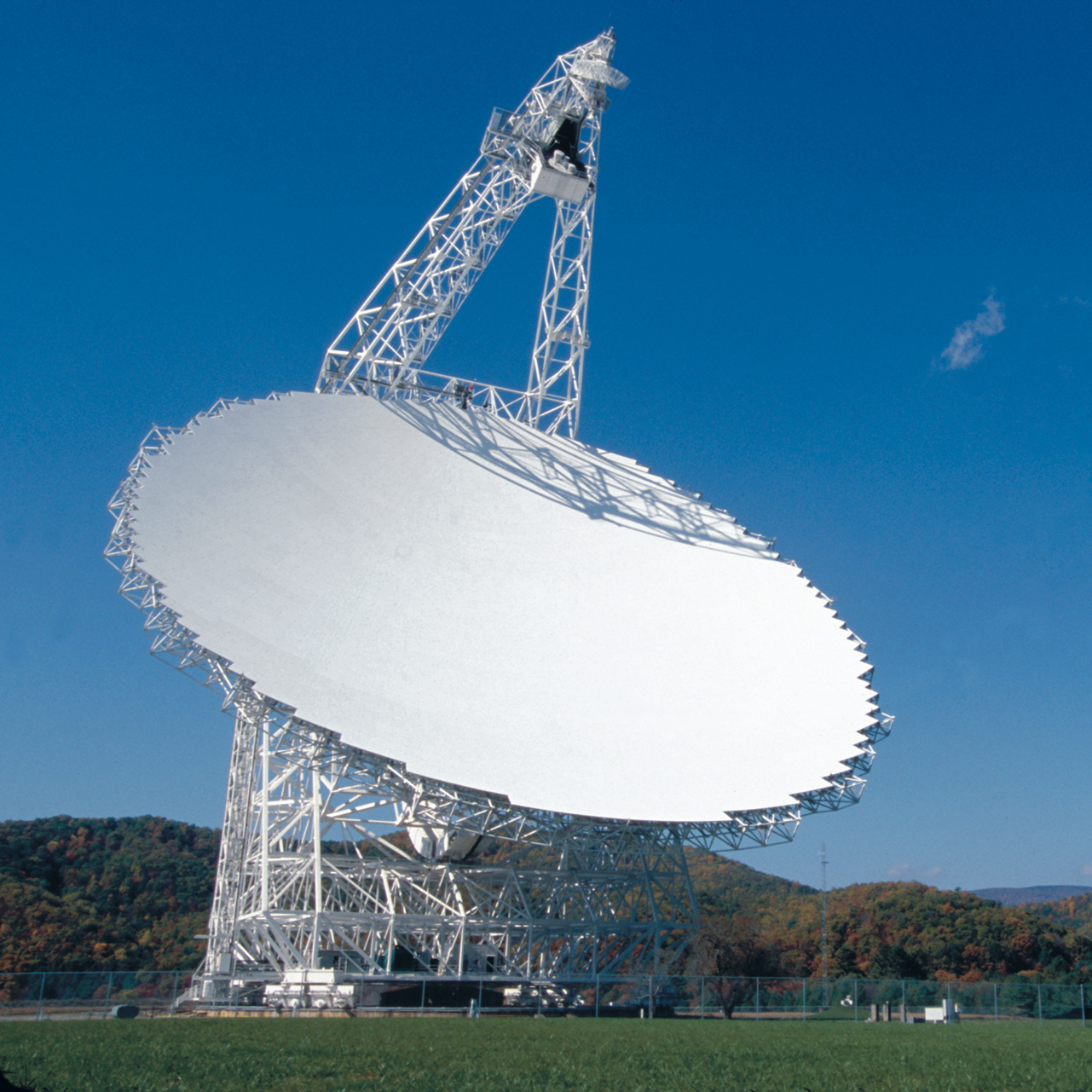
The Green Bank Telescope (100m diameter) operates at radio wavelegths. Credit: NRAO/AUI/NSF
- Another way is to work at higher frequencies (shorter wavelengths), e.g. sub-mm radio astronomy (IRAM 30m telescope)
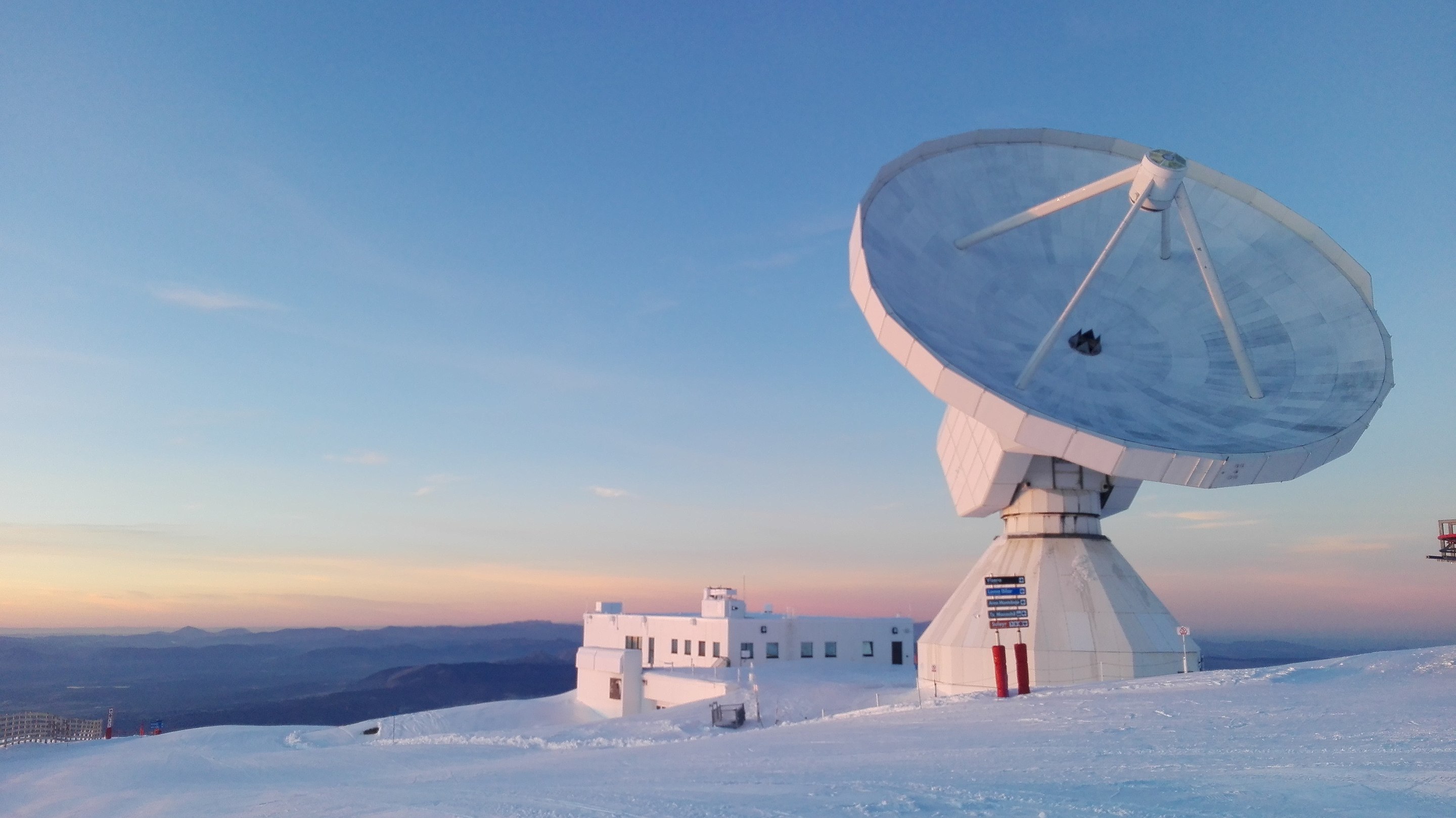
The IRAM 30m diameter telescope, which operates at sub-mm wavelengths. Credit: Wikipedia/IRAM-gre
- A final way is to use interferometry, sometimes also at sub-mm wavelengths (ALMA), which will be the main focus of this course
It’s easier to build larger telescopes at longer wavelengths because the tolerances required for the reflecting surface are less strict than at optical wavelengths. Though typically one must keep surface tolerances to within $$ \sigma = \frac{\lambda_\mathrm{min}}{16}, $$ otherwise the efficiency of the antenna starts to decline substantially. For the 100 m diameter GBT operating at it’s highest frequency (100 GHz) or 3 mm, this translates to \(200\;\mu\mathrm{m}\), which is the thickness of two sheets of paper! That’s quite an engineering challenge, and is the reason why large, steerable dishes are difficult to build.
Keeping telescopes fixed is one way to build a little bit bigger, such as FAST, which is a five hundred meter diameter fixed telescope in China. See also Arecibo, which unfortunately collapsed in December 2020. Eventually, though, the materials/engineering cost to building large single dish telescopes becomes prohibitive.
Single dish observations
The “beam” of a receiving antenna, or power pattern as a function of direction, can be calculated using the reciprocity theorems for transmitting and receiving antennas. These state that the far field electric field pattern \(f(l)\) is the Fourier transform (much more in lectures 2 and 3!) of the electric field illuminating the aperture of the telescope \(g(u)\).
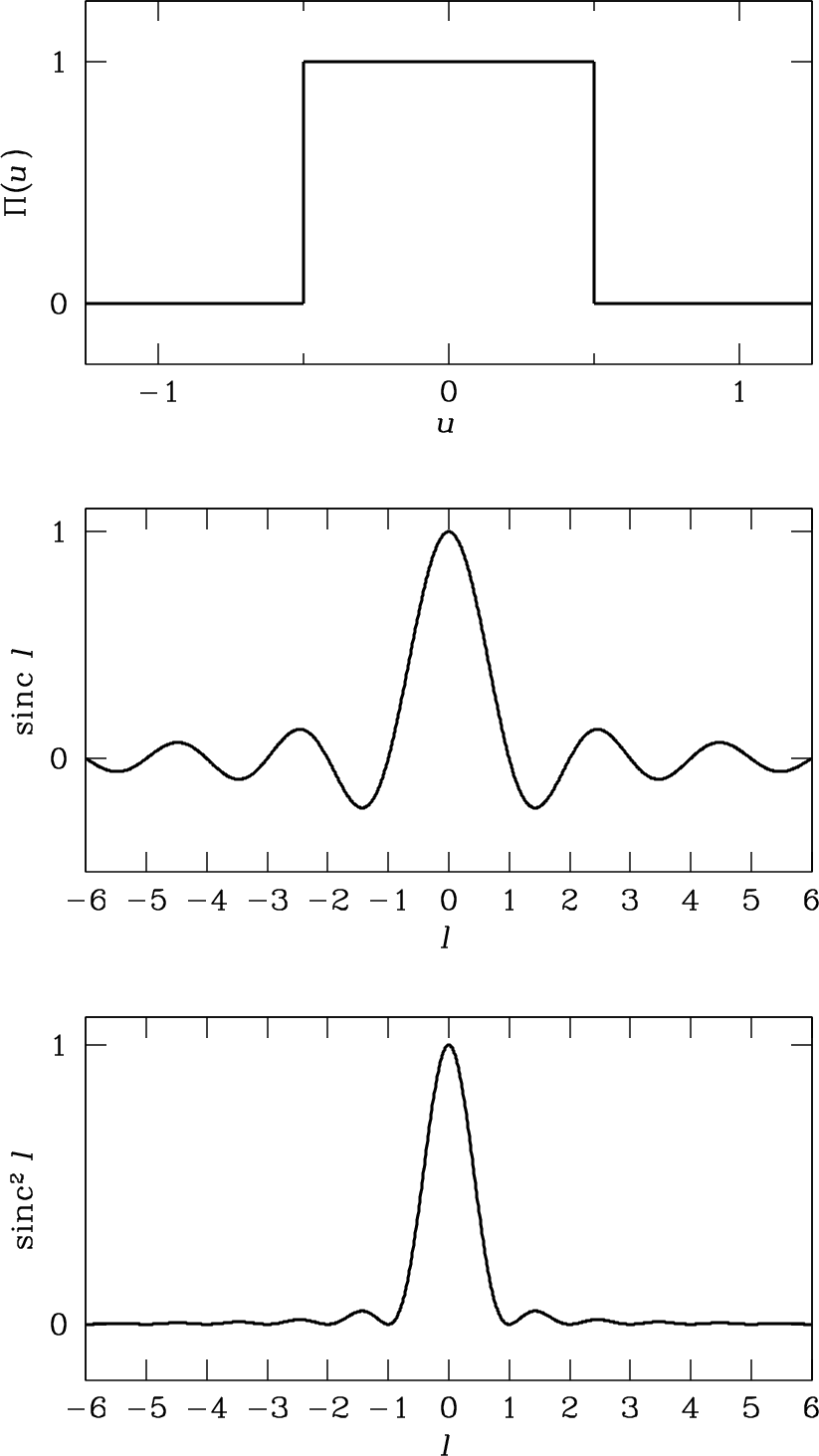
A schematic illustration of (top): Uniformly illuminated aperture (middle): The electric field pattern of the antenna, as a function of direction (bottom): The power pattern of the antenna, as a function of direction. Credit: Essential Radio Astronomy
For large apertures, the nulls at \( l = \pm 1, 2, \ldots\) appear at the angles \(\theta \approx \lambda/D, 2 \lambda/D, \ldots\). In two dimensions, for a circular aperture, this is an Airy pattern.
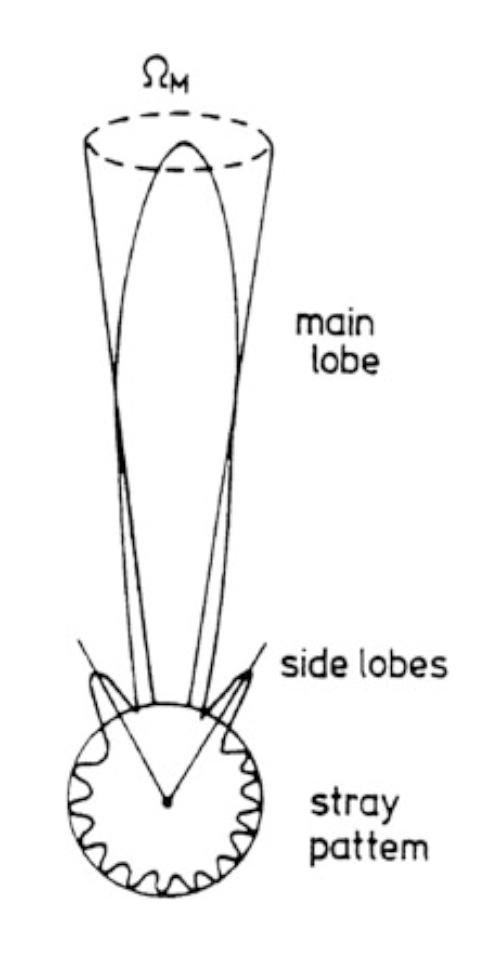
A beam power pattern plotten in polar coordinates, demonstrating that the antenna can pick up power from sidelobes at range of angles. Credit: Tools of Radio Astronomy.
This is an idealized representation, but is still helpful. The beam can pick up power through sidelobes at a range of angles. Directional antennas help concentrate power in the main beam, but antennas with secondary stages (and thus supports, like most telescopes) create opportunities for ground radiation to reflect into the receiver.
You can think of single-dish telescopes (unless they have a sophisticated, multi-pixel receiver) essentially as single-pixel devices. So to make a map of the sky, you would need to raster scan the telescope across the region of interest, reading out antenna temperature as a function of RA, Dec. To make a good (i.e., scientifically accurate) map, you should focus on Nyquist sampling the sky to a uniform sensitivity, usually through a hexagonal pattern of dithering. More advanced instruments may have an array of “feeds” in a focal plane (mirroring a set of “pixels”), but this is still a small number of pixels compared to a typical CCD (e.g., 25 or 36 compared to \(2046^2\)).
Image Units
Radiative transfer recap
What are the units of the sky, and the images we make as representations of it?
One of the most useful quantities from radiative transfer is \(I_\nu\).
\(I_\nu \) is the specific intensity of radiation, you can think of it as the energy carried along by an infinitesimal “bundle” of rays.
It has dimensions of: $$ \mathrm{energy}\; (\mathrm{time})^{-1} \;(\mathrm{area})^{-1} \;(\mathrm{solid\,angle})^{-1} \; (\mathrm{frequency})^{-1} $$ in CGS units, we would write $$ \mathrm{ergs}\;\mathrm{s}^{-1}\;\mathrm{cm}^{-2}\;\mathrm{ster}^{-1}\;\mathrm{Hz}^{-1} $$ In astronomical settings, I’ve always seen \(I_\nu\) referred to as the “specific intensity.” In non-astronomy settings, I’ve seen “spectral intensity.” If \(I_\nu\) is integrated over all frequencies, it’s called the radiant intensity \(I\).
\(I_\nu \) can be a little mind-bending to think about… it can be a function of
- 3D space \(\vec{x}\)
- direction \(\vec{\Omega}\)
- frequency
Intensity itself is not a vector quantity; rather it is a scalar field that is function of position and direction \(I_\nu(\vec{x}, \vec{\Omega})\). Rybicki and Lightman write the angular direction vector as \(\vec{\Omega}\) and the solid angle surrounding that vector as \(\mathrm{d}\Omega\).
The geometry surrounding the concept of specific intensity. The normal vector is \(\vec{\Omega}\), the position \(\vec{x}\) in 3D space corresponds to the location of the \(dA\) patch. The Credit: Radiative Processes, Figure 1.2
If we have a defined reference frame, we would probably write \(\vec{\Omega}\) as a vector in spherical coordinates and define the components along \(\hat{\phi}\) and \(\hat{\theta}\) and let \(\mathrm{d}\Omega = d\phi \sin \theta d\theta\).
When we are making astrophysical observations from the earth, though, we are making or acquiring images of regions of the celestial sky. So we generally talk of \(I_\nu(\alpha, \delta)\), where \(\alpha\) and \(\delta\) are R.A. and declination offsets from some direction, respectively. We’re always looking from the same place (at least compared to the size of the universe), so we don’t worry about specifying position within 3D space. But if we went to the Andromeda Galaxy and started mapping the celestial sky, we would need to, then. In the end though, images are have the same units because they represent specific intensity. It’s very common to refer to \(I_\nu(\alpha, \delta)\) as the surface brightness.
When we’re discussing images of astronomical sources, we’re usually using RA \(\alpha\) and Dec \(\delta\). A solid angle simply describes the area on a unit sphere (e.g., the sky), the area itself need not be circular. The Very Large Array, located in Socorro, NM. Credit: NRAO
Flux
Once you’ve defined \(I_\nu\), then it’s relatively easy to calculate quantities like energy density, flux, momentum, etc, as integrals of the specific intensity field.
Flux is where you integrate out the angular dependence:
$$ F_\nu = \int I_\nu \cos \theta d \Omega $$ (intensity passing through some differential area \(dA\), lowered by the effective angle).
\(F_\nu\) has units of $$ \mathrm{ergs}\;\mathrm{s}^{-1}\;\mathrm{cm}^{-2}\;\mathrm{Hz}^{-1} $$ (i.e., angular dependence has been integrated out).
Most astrophysical sources produce significantly less energy in radio waves compared to higher frequency bands, and so the raw CGS unit can be quite cumbersome. To make this easier, astronomers use a unit called the “Jansky,” which is defined as
$$ 1\,\mathrm{Jy} = 10^{-23}~\mathrm{ergs}\;\mathrm{s}^{-1}\;\mathrm{cm}^{-2}\;\mathrm{Hz}^{-1} $$
The Jansky is a unit of flux.
How do we report specific intensities/surface brightnesses for radio sources, then? We can, reintroduce the “per solid angle” to the Jansky, for example $$ \mathrm{Jy}\;\mathrm{arcsec}^{-2}. $$
Later on the course, we’ll talk about \(\mathrm{Jy}\;\mathrm{beam}^{-1}\), which another unit of surface brightness/specific intensity.
Other units of surface brightness that you might encounter at other wavelengths include \(\mathrm{mag}\;\mathrm{arcsec}^{-2}\) (optical) and \(\mathrm{MJy}\;\mathrm{sr}^{-1}\) (infrared).
Questions for review:
- What is the name of \(I_\nu\), and what are its units?
- What is the name of \(F_\nu\), and what are its units?
- If we made an astronomical observation of a “point source,” would we report \(I_\nu\) or \(F_\nu\)?
- What about for a spatially resolved source?
- Is a Jansky a unit for \(I_\nu\) or \(F_\nu\)?
Using \(F_\nu\) and \(I_\nu\) to represent point sources and spatially resolved sources, respectively. Credit: Ian Czekala
The many temperatures of radio astronomy
From Cosmic Sources only
- brightness temperature: \(T_b\), the temperature corresponding to the specific intensity if we used the full form of the Planck formula $$ I_\nu = \frac{2 h \nu^3}{c^2} \frac{1}{\exp{(h \nu / k T_b)} - 1} $$
- antenna temperature: the temperature corresponding to the specific intensity if we were in the Rayleigh-Jeans domain. Added benefit that specific intensity is linearly related to antenna temperature and makes it easy to substitute one for the other. $$ T_A(\nu) = \frac{c^2}{2 k \nu^2} I_\nu $$
In the field of radio astronomy, be aware that one frequently combines temperatures in other interesting ways. One can express random noise power in terms of an effective temperature $$ P = k T \Delta \nu $$ where \(\Delta \nu\) is the bandwidth of the observation. Here the power is equal to the noise power delivered to a matched load by a resistor at physical temperature \(T\). By matched load, we mean we connect a resistor to the input terminals of a linear amplifier. The fact that this resistor has some temperature (i.e., we haven’t cooled it to absolute zero…) means that the thermal motion of the electrons will produce a random, variable current \(i(t)\) input to the amplifier. The mean value of this current is zero, but the root mean squared value is non-zero, and this represents a non-zero power. I.e., you can draw (some) power from a resistor at room temperature, purely from thermal motions. The situation is not dissimilar to the random walk of a particle in Brownian motion. For more details, see Tools of Radio Astronomy, Chapter 1.8.
Including noise sources
- Antenna temperature \(T_A\) the component of the power received by the antenna from cosmic sources. It has the same interpretation as before (though we’ll talk about beam dilution in a second).
- Receiver temperature \(T_R\) the component of the power from internal noise of the receiver components themselves, ground radiation, atmospheric emission, etc…
- System temperature \(T_S = T_A + T_R\) is the sum of receiver temperature and antenna temperature. It’s the one power number coming out of the backend of your telescope. It’s up to you to calibrate \(T_R\) accurately enough to measure \(T_A\).
In any observation, you will have your cosmic signal of interest and several contributions of noise (see Essential Radio Astronomy, Ch. 3.6.1) $$ T_S=T_\mathrm{cmb}+T_\mathrm{rsb}+T_A + [1−\exp(−\tau_A)] T_\mathrm{atm}+T_\mathrm{spill}+T_r+ \ldots $$ such as the CMB, other galactic background sources, the atmosphere, spillover radiation from the ground, the temperature of the radiometer itself (hopefully cryogenically cooled), etc.
In the limit that \(T_A \ll T_S\) (most astronomy situations, unfortunately!), we have $$ S/N \approx C \frac{T_A}{T_S} \sqrt{\Delta \nu \Delta t} $$ where \(C\) is a constant of proportionality greater than or equal to 1, and \(\Delta t\) is the integration time. If we let \(\Delta \nu \approx 1\;\mathrm{GHz}\) and \(\Delta t \approx 1\;\mathrm{h}\), then we can get \(\sqrt{\Delta \nu \Delta t} \approx 10^6\), allowing us to detect a signal which is less than \(10^{-6}\) the system noise. A great illustration of this capability is the COBE satellite that studied CMB anisotropies with brightness temperatures \(< 10^{-7}\) that of the system temperature. To achieve these contrasts, however, it’s important to keep systematics under control, otherwise the S/N scaling won’t hold!
Beam dilution
In previous lectures, we’ve been talking about specific intensity \(I_\nu(\Omega)\) as a “known” quantity of direction (e.g., R.A., Dec.) and used antenna temperature \(T_A\) as a linear proxy for its specification. For the following discussion, we’re going to move into the realm of observations, and discuss the ways \(T_A\) can be an unfaithful proxy for the “true” specific intensity distribution or brightness temperature. we’ll use the symbol \(T_b(\Omega)\) to denote the “true” brightness/antenna temperature, assuming we’re in the Rayleigh-Jeans limit, and redefine \(T_A\) to mean the response of the telescope to the cosmic radiation.
When we’re doing observations, we don’t always have access to the highest resolution version of \(T_b(\Omega)\), but rather we have access to a quantity which is the true \(T_b(\Omega)\) convolved with the beam of the telescope, which is the implication of \(T_A\) for this discussion.
When astrophysical sources are insufficiently resolved, our measurements of \(I_\nu\) do not trace the true sky distribution, specifically features are smeared out over a spatial extent and peak intensities are reduced. This means that using these insufficiently resolved measurements of \(T_A\) will not accurately trace the true underlying temperatures of the astrophysical source (even if the emission from the source is actually thermal in origin). Of course, we never have infinite spatial resolution, so there will always be structure on scales beyond that of our observations. Credit: Ian Czekala
large (fully resolved) source
In the limit that we are observing a source that subtends a solid angle much larger than the beam of the antenna, $$ \Omega_S > \Omega_A $$ the convolution of the beam doesn’t matter, we’re still sensing approximately the same \(T_b(\Omega)\) such that $$ T_A(\Omega) \approx T_b(\Omega). $$ If the source is in LTE, then we also have that \(T_A \approx T\).
small (unresolved) source
If the source is more compact than the antenna beam, $$ \Omega_S < \Omega_A, $$ then the measured antenna temperature is basically the “true” intensity averaged over the area of the main beam. This lowers the measured antenna temperature by a factor $$ \frac{T_A}{T_b} = \frac{\Omega_S}{\Omega_A} $$ where the ratio \(\frac{\Omega_S}{\Omega_A}\) is called the beam filling factor.
For example, you could have a compact source with \(T_b = 10^4\) K, but if it only fills 1% of the beam solid angle then you would measure an antenna temperature of 100 K. If you took your observations at face-value (and assumed LTE), then you would incorrectly conclude that the source is 100x cooler than it actually is.
Beam dilution also applies to observations of sources that have structure on spatial scales below the observable limit, which, to be honest, is going to be most astrophysical sources of interest. For example, consider a gas filament in a star-forming region.
Radio-bright, spatially concentrated regions will be “smeared out” by the beam. If you wanted to use antenna temperature (and assume LTE) to estimate the physical conditions of the gas filament, you do so at the peril of measuring incorrect temperatures. The unfortunate reality here is that, without higher resolution images to guide you (which sometimes exist at optical or infrared wavelengths), it’s quite difficult to estimate how badly your measurements are affected by beam dilution.
For more useful single-dish guidance, see these notes by James Jackson, or Ch 3.1.6 of Essential Radio Astronomy.
Introduction to interferometric arrays, ALMA, VLA, SMA, VLBA
Now that we’ve covered some of the fundamentals around radio telescopes and single-dish antennas, we’ll move on to discussing how we combine the signals from multiple antennas to do interferometry. Here are some of he interferometers operating today:
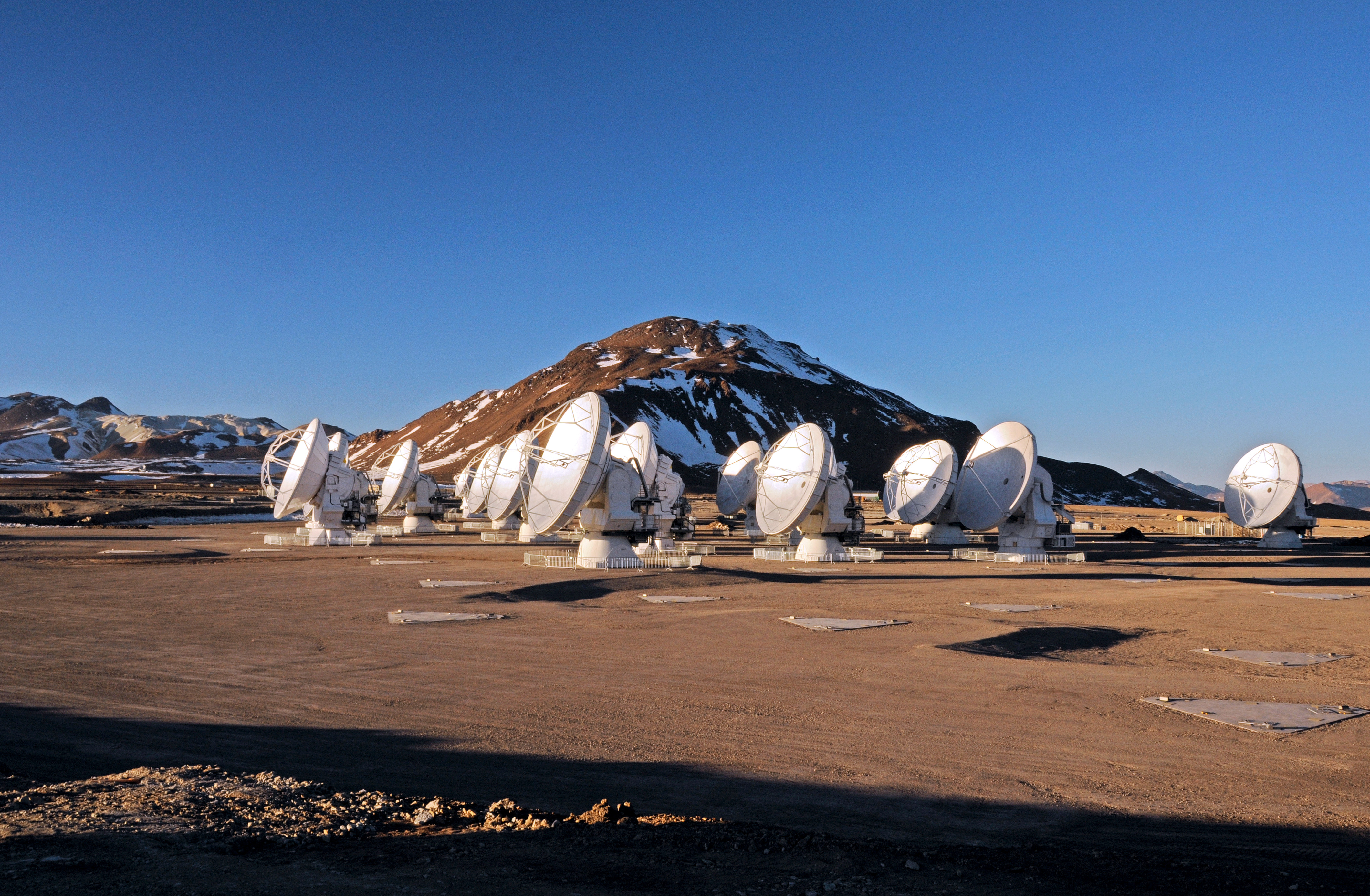
The Atacama Large (Sub)millimeter Array, an interferometric array of 66 antennas operating at sub-millimeter wavelengths. The largest antennas in the array are only 12m in diameter, yet through interferometry, the array is able to obtain far higher spatial resolution than the largest single-dish antennas. Credit: NRAO/ESO/NAOJ/JAO
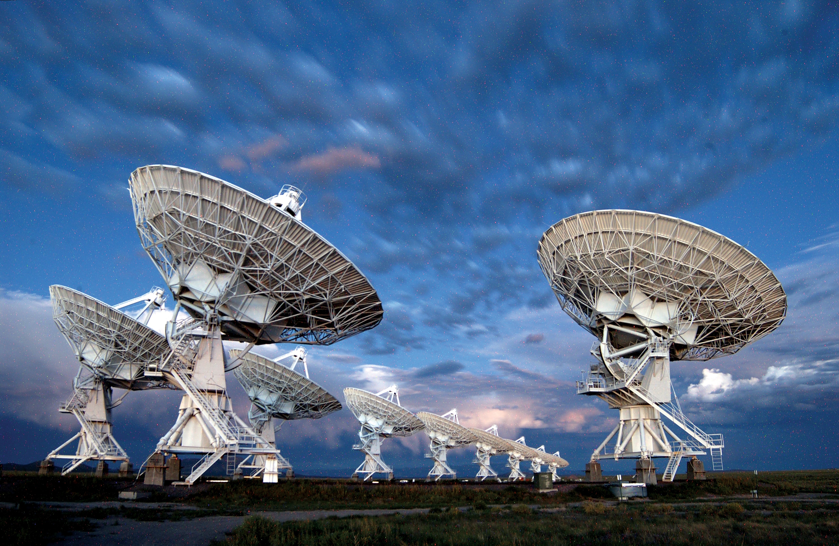
The Very Large Array, located in Socorro, NM. Credit: NRAO
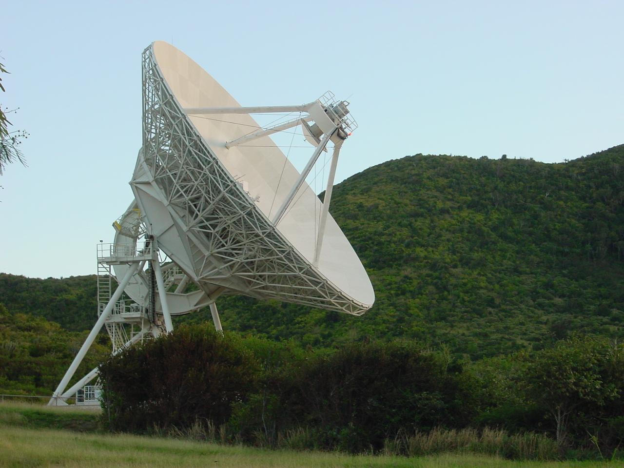
One antenna at the Eastern end of the Very Long Baseline Array (VLBA), St. Croix, U.S. Virgin Islands. Credit: Cumulus Clouds
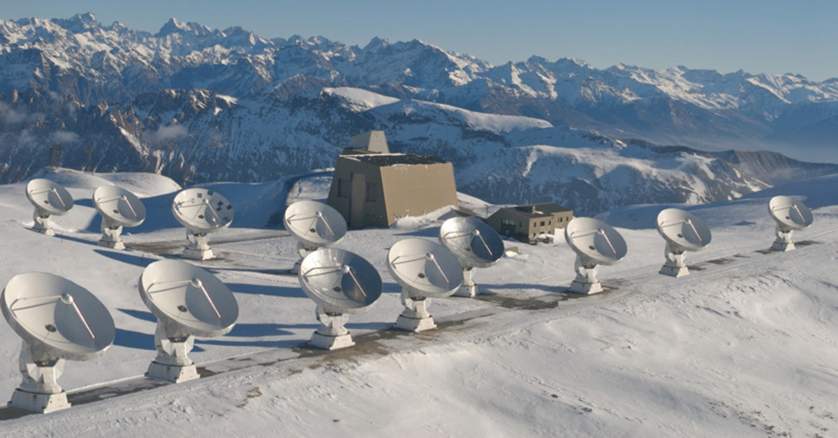
The NOEMA, located in the French Alps on the Plateau du Bure. Credit: IRAM/Rebus
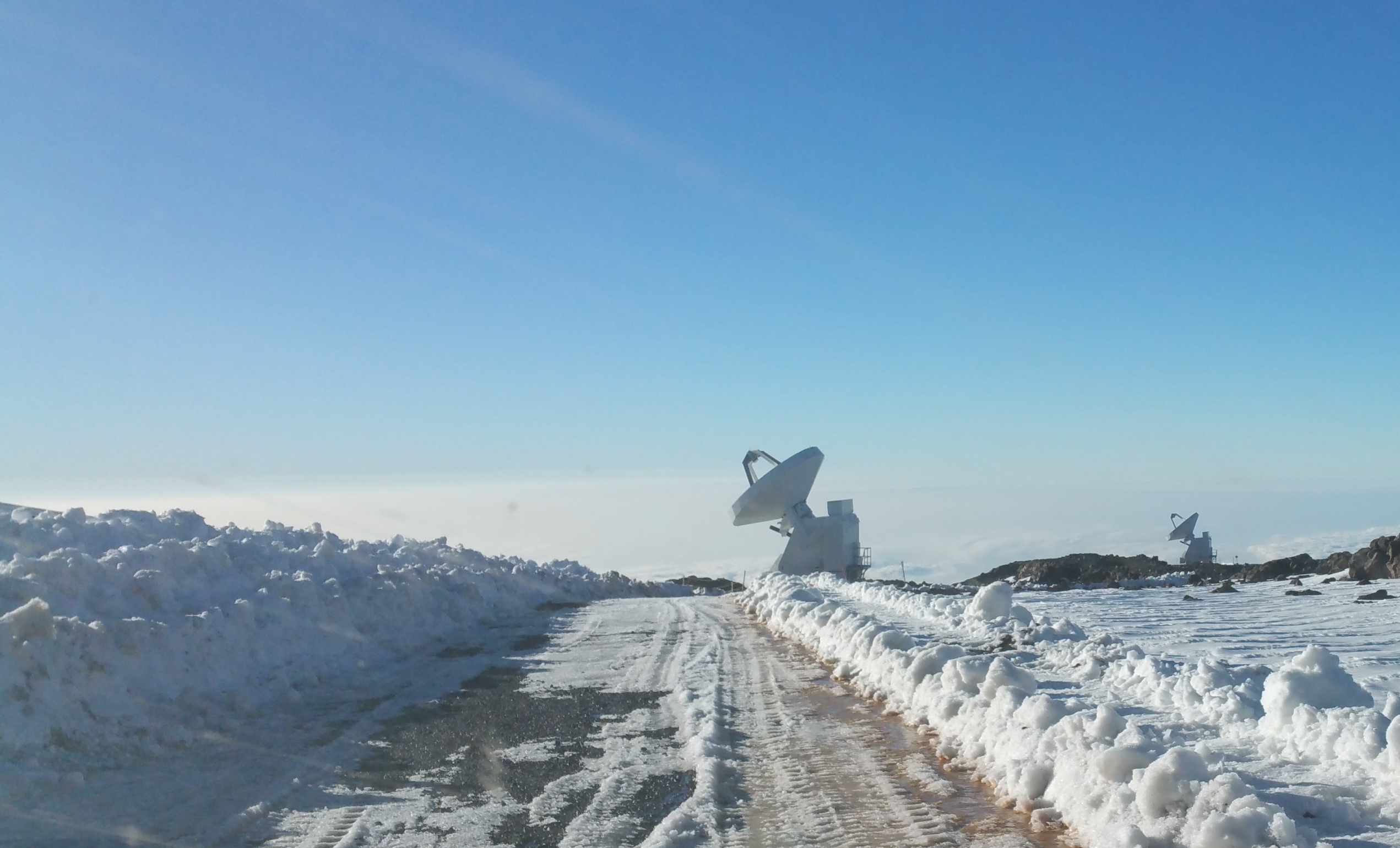
The Submillimeter Array (SMA), located on Mauna Kea, Hawaii. Credit: I. Czekala