The Fourier Transform I
Reference Materials for this lecture:
- The Fourier Transform and its Applications by R. Bracewell
- Interferometry and Synthesis in Radio Astronomy by Thompson, Moran, and Swenson, particularly Appendix 2.1
- Fourier Analysis and Imaging by R. Bracewell
Useful (and entertaining!) introductions to the topic:
- Youtube: 3Blue1Brown
Complex Numbers
A complex number \(z\) is one in the form of \(z = a + b i\), where \(i\) is the imaginary unit. The imaginary unit satisfies the equation $$ i^2 = -1. $$
So a complex number has both real (\(a\)) and imaginary (\(b\)) components to it. We can represent this as a plot on the Cartesian plane:

Representation of a complex number on the Cartesian plane. Credit: Wolfkeeper
Alternatively, we can also represent a complex number on the polar plane, using an amplitude \(r\) and phase \(\varphi\):

Representation of a complex number on the polar plane. Credit: Kan8eDie, based on Wolfkeeper
$$ z = r e^{i \varphi} = r (\cos \varphi + i \sin \varphi). $$
This is closely related to Euler’s formula $$ e^{i x} = \cos x + i \sin x $$ for a complex sinusoid. It’s useful to keep in mind Euler’s identity: $$ e^{i \pi} + 1 = 0. $$
It’s possible to convert from the Cartesian form to polar form and vice-versa:
$$
r = |z| = \sqrt{a^2 + b^2}
$$
and
$$
\varphi = \arg(z) = \arg(a + bi)
$$
which is most easily carried out using the arctan2 function, to avoid quadrant ambiguities.
$$
\varphi = \mathrm{arctan2}(b, a).
$$
You can go from polar back to Cartesian by writing $$ z = r e^{i \varphi} = r (\cos \varphi + i \sin \varphi) $$ and then doing $$ a = \Re(z) = r \cos \varphi $$ and $$ b = \Im(z) = r \sin \varphi. $$
The Fourier Transform
References include a mix of
- Ch 2 of The Fourier Transform and its Applications by R. Bracewell
- Appendix 2.1 of Interferometry and Synthesis in Radio Astronomy by Thompson, Moran, and Swenson
First, we’ll introduce the equations and then explain what’s going on.
Forward transform: $$ F(s) = \int_{-\infty}^{\infty} f(x) e^{-i 2 \pi x s}\,\mathrm{d}x $$ also called the “minus-\(i\)” transform.
Inverse transform: $$ f(x) = \int_{-\infty}^{\infty} F(s) e^{i 2 \pi x s}\,\mathrm{d}s $$ also called the “plus-\(i\)” transform.
Note that there are alternate conventions for the Fourier transform pairs, which vary as to whether the \(2 \pi\) factor appears in the exponent or as a pre-factor. We prefer the notation we’ve provided here because we find it much easier to keep track of \(2\pi\) factors.
Successive transforms:
We can show that $$ f(x) = \int_{-\infty}^{\infty} \left [ \int_{-\infty}^{\infty} f(x) e^{-i 2 \pi x s}\,\mathrm{d}x \right ] e^{i 2 \pi x s}\,\mathrm{d}s, $$ i.e., successive transformations yield back the original function. We don’t have time to walk through the proof, but it’s available in TMS Section A2.1.
Therefore, we have $$ f(x) \leftrightharpoons F(s), $$ where the \(\leftrightharpoons\) denotes a Fourier transform pair. Sometimes you might also see the notation \(\leftrightarrow\). Generally, if we have functions like \(f\) or \(g\), then we denote their Fourier transform pairs with captial letters (e.g., \(F\), \(G\))).
How to think about the domains The Fourier transform maps domains from \(x\) to \(s\), where \(s\) has units of “cycles per unit of \(x\)”. E.g., if \(x\) is in units of time (seconds), then \(s\) has units of cycles/second, commonly known as hertz. The FT can also be applied to spatial distance coordinates (e.g., \(x\) in meters) and spatial coordinates on the sky (e.g., \(x\) in arcseconds).
So let’s say someone is playing a chord on a musical instrument. If \(f(x)\) represents the time-series of pressure values near your ear, then \(F(s)\) represents the notes that are being played (we would probably be most interested in something like \(|F(s)|^2\) for power as a function of frequency, like a spectrogram).
Conditions on existence
Given the strong evidence via physical systems that the Fourier transform of particular time-series exists (e.g., spectrums for waveforms, antenna radiation patterns), there are actually some mathematical functions whose Fourier transforms do not exist.
Physical possibility (in physical systems) is a sufficient condition for the existence of its transform.
Sometimes, though, we consider waveforms like
- \(\sin(t)\): harmonic wave
- \(H(t)\): Heaviside step
- \(\delta(t)\): impulse
Strictly speaking, none of these functions has a Fourier transform. What do we mean that they do not have Fourier transforms? $$ F(s) = \int_{-\infty}^{\infty} f(x) e^{-i 2 \pi x s}\,\mathrm{d}x $$ does not converge for all values of \(s\). Consider \(\sin(t)\) integrated from \((-\infty, \infty)\)… it’ll just keep oscillating about 0.
None of these waveforms are actually physically possible, though, because a waveform \(\sin(t)\) would have need to been switched on an infinite time ago, a step function would need to be maintained for an infinite time, and an impulse would need to be infinitely large for an infinitely short time.
So, what are the conditions for the existence of Fourier transforms.
- The integral of \(|f(x)|\) from \(-\infty\) to \(\infty\) exists.
- Any discontinuities in \(f(x)\) are finite.
In a physical circumstance, these conditions would be violated when there is infinite energy.
Transforms in the limit
Though we just outlined functional forms whose Fourier transforms do not strictly exist, we can find a way to think such that the transforms of these functions do exist in a practical sense. This is by considering them in the limit.
Consider a periodic function whose transform would strictly not exist, such as \(P(x) = \sin(x) \), since $$ \int_{-\infty}^\infty |P(x)|\,\mathrm{d}x $$ would not converge.
We could modify this function ever so slightly by multiplication with a very broad Gaussian envelope \(\exp(-\alpha x^2)\), where \(\alpha\) is a small positive number, then this modified version may have a transform. As we let \(\alpha \rightarrow 0\), then we approach \(P\) in the limit. $$ \int_{-\infty}^\infty |e^{-\alpha x^2} P(x)|\,\mathrm{d}x $$
As \(\alpha \rightarrow 0\) the transform may still not exist for all \(s\), however, we can still be quite productive with the sequence of transforms that do exist as we approach this limit. Therefore, we can practically use the Fourier transform for all physical systems that we might consider. We’ll revisit this in more detail when we talk about Fourier series, line spectra, and the sampling theorem.
Oddness, Evenness, and Complex Conjugates
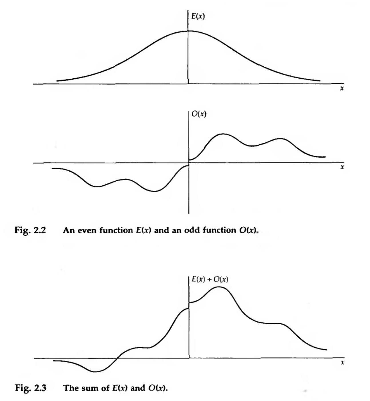
An even function \(E(x)\) and an odd function \(O(x)\), followed by their sum. Credit: The Fourier Transform and Its Applications, Bracewell, Figs 2.2 and 2.3.
Even functions have $$ E(-x) = E(x) $$ and are symmetrical.
Odd functions have $$ O(-x) = -O(x) $$ and are antisymmetrical.
The sum of even and odd functions is, in general, neither even nor odd.
Any function \(f(x)\) can be split unambiguously into it’s odd and even parts, though, where $$ E(x) = \frac{1}{2} \left [ f(x) + f(-x) \right] $$ and $$ O(x) = \frac{1}{2} \left [ f(x) - f(-x) \right] $$ and so we have $$ f(x) = E(x) + O(x), $$ where both \(E\) and \(O\) are in general complex-valued.
Evenness and oddness are very useful because we can these definitions to re-write the Fourier transform as $$ F(s) = 2 \int_0^\infty E(x) \cos(2 \pi x s)\,\mathrm{d}x - 2 i \int_0^\infty O(x) \sin (2 \pi x s)\,\mathrm{d}x. $$
We see that
- If a function is even, its transform is even
- If a function is odd, its transform is odd
and other results summarized by Bracewell in Chapter 2:
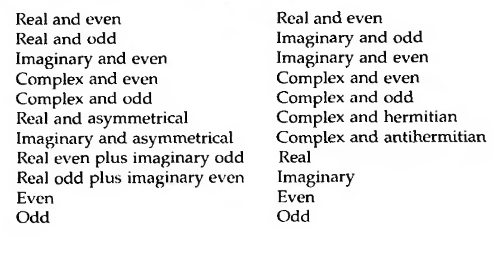
If a function has the characteristics in the left column, then its Fourier transform has the characteristics in the right column. Credit: Bracewell Ch. 2
These relationships are extremely useful for quickly ascertaining the basic nature of the Fourier transform of any function you may encounter, as well as planning how to numerically compute transforms using fft or rfft packages.
Complex conjugates
If we have the complex conjugate of function \(f(x)\), denoted by \(f^*(x)\), then we have
$$ f^{*}(x) \leftrightharpoons F^{*}(-s) $$
Transforms of some simple functions
Let’s practice by taking the Fourier transforms of some functions.
Boxcar
The rectangle or “boxcar” function is The rectangle, or boxcar function. Credit: Bracewell Ch. 3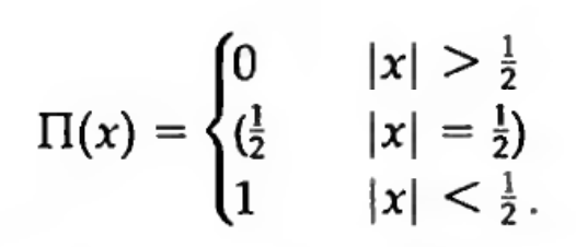
Let’s calculate the Fourier transform. The function itself is simple, so this is mainly an exercise in choosing the right limits $$ F(s) = \int_{-\infty}^{\infty} f(x) e^{-i 2 \pi x s}\,\mathrm{d}x $$
$$ F(s) = \int_{-1/2}^{1/2} e^{-i 2 \pi x s}\,\mathrm{d}x $$
We can use Euler’s formula to write $$ F(s) = \int_{-1/2}^{1/2} \cos(2 \pi x s) + i \sin(2 \pi x s) \,\mathrm{d}x $$ and visually seen that the \(\sin\) term would eventually cancel itself out, or we could have relied upon the fact that we know \(\Pi(x)\) is an even function (\(O(x) = 0\)) and used $$ F(s) = 2 \int_0^\infty E(x) \cos(2 \pi x s)\,\mathrm{d}x - 2 i \int_0^\infty O(x) \sin (2 \pi x s)\,\mathrm{d}x. $$ to yield $$ F(s) = 2 \int_0^{1/2} \cos(2 \pi x s)\,\mathrm{d}x $$
$$ F(s) = 2 \Big |_0^{1/2} \frac{\sin 2 \pi x s}{2 \pi s} = \frac{\sin \pi s}{\pi s} = \mathrm{sinc}(s) $$
Note that we (and Bracewell) define $$ \mathrm{sinc}(s) = \frac{\sin \pi s}{\pi s} $$ this is called the normalized sinc function, and (IMO) is the most useful because of it’s nice Fourier pair relationships. There is also the “unnormalized” sinc function, which doesn’t have the factors of \(\pi\) in it, but we won’t use that in this course. The normalized sinc function has the properties that
- its peak is equal to 1 \(\mathrm{sinc}(0) = 1\)
- its “nulls” are located at non-zero integer values of \(n\) for \(\mathrm{sinc}(n)\)
- its integral from \(-\infty,\infty\) is equal to 1
So we have the Fourier pair: $$ \Pi(x) \leftrightharpoons \mathrm{sinc}(s) $$ The unit rectangle (or boxcar) function has the Fourier transform pair of a normalized sinc function.
This is also the same relationship that we introduced in the first lecture: the far field electric field pattern (sinc) is the Fourier transform of the electric field illuminating the aperture of the telescope (boxcar).
Gaussian
How about the Fourier transform of a Gaussian function? $$ f(x) = \exp \left ( -\frac{x^2}{2 a ^2} \right ) $$
$$ F(s) = \int_{-\infty}^{\infty} \exp \left ( -\frac{x^2}{2 a ^2} \right ) \exp (-i 2 \pi x s)\,\mathrm{d}x $$
$$ F(s) = \int_{-\infty}^{\infty} \exp \left ( -\frac{x^2}{2 a ^2} -i 2 \pi x s \right )\,\mathrm{d}x $$
Usually, when I see something like this, my standard approach is to start browsing books of integrals like Gradshteyn and Ryzhik for ideas about how I might rearrange the integrand and successfully evaluate the integral. I’d usually just go for this. But, in this case, we can actually do something using a trick you probably learned in jr. high school, called completing the square.
Ok, so we’ve got terms in the exponent with \(x^2\) and \(x\), and an equation that looks like $$ a x^2 + bx + c = 0 $$ which we want to turn into something that looks like $$ a(x + d)^2 + e = 0. $$
The answer is that $$ d = \frac{b}{2a} $$ and $$ e = c - \frac{b^2}{4 a} $$ such that our rearranged exponent becomes $$ -\left [ \frac{x^2}{2 a ^2} + i 2 \pi x s \right ] = -[(x - 2i \pi a^2 s)^2 + 4 \pi^2 a^4 s^2]/2a^2 $$ Why was this useful? Well, the integral is over \(x\), so we can pull out all terms that do not depend on \(x\), giving us a rearranged integral of $$ F(s) = \exp(-2 \pi^2 a^2 s^2 ) \int_{-\infty}^\infty \exp \left (-\frac{(x - 2 i \pi a^2 s)^2}{2 a^2} \right)\,\mathrm{d}x $$
Here it is helpful to remember your Gaussian integration formulas such that $$ \int_{-\infty}^\infty e^{-a(x + b)^2}\,\mathrm{d}x = \sqrt{\frac{\pi}{a}}. $$
Thus, the integral contributes another factor of \(\sqrt{2 \pi} a\) and the final result is
$$ F(s) = \sqrt{2 \pi} a \exp(-2 \pi^2 a^2 s^2 ) $$
What functional form is this? This is another Gaussian, though the normalization and standard deviation are a bit different! So, we see that the Gaussian function is a Fourier transform pair with itself.
Hopefully now you have a taste of how to compute Fourier transforms. At its most basic, it’s just a matter of setting up and evaluating the integral. For many function forms, you can use integration strategies to arrive at analytic solutions. As a practical matter, in the next lecture we’ll see how we can evaluate this integral numerically.
Convolution
The convolution of two functions \(f(x)\) and \(g(x)\) is defined as $$ \int_{-\infty}^\infty f(u) g(x - u)\,\mathrm{d}u $$ and is frequently written using the \(*\) symbol. The convolution produces a new function, so we have $$ h(x) = f(x) * g(x). $$
Convolution as a process is very useful to think of graphically
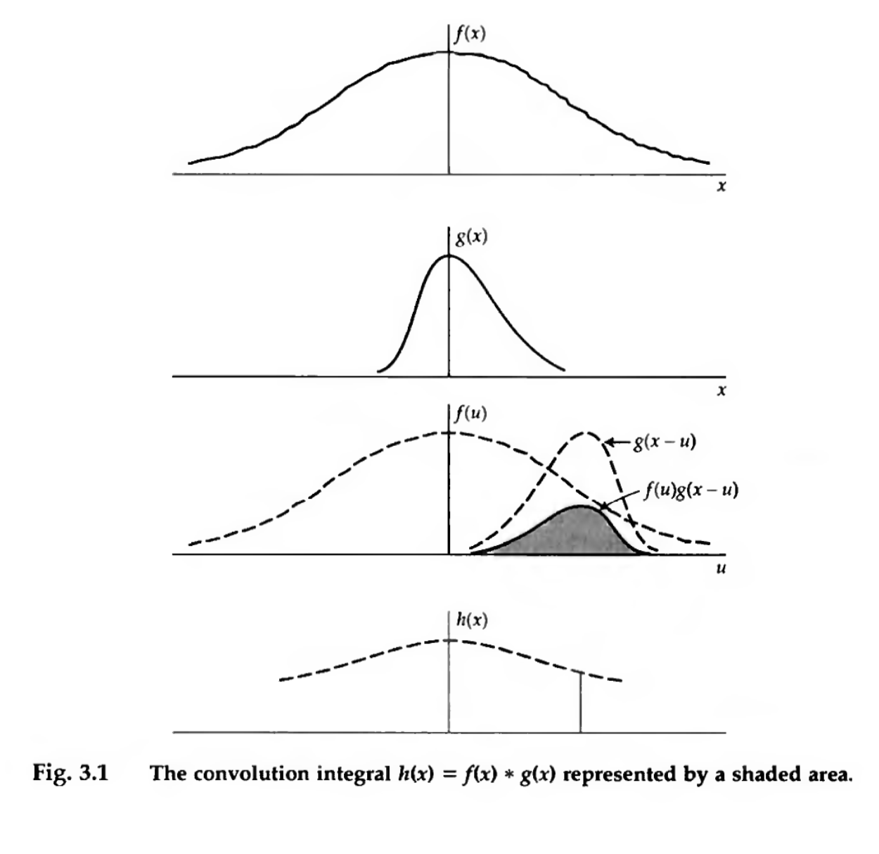
A graphical representation of the convolution of two functions \(f(x)\) and \(g(x)\). The \(g\) function is flipped, shifted to \(x\), and then multiplied against \(f\). The value of the convolution \(h(x)\) is given by the integral of the multiplied product. Credit: Bracewell Ch. 3
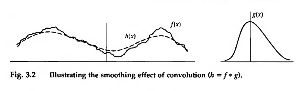
In general, convolution by most functions (e.g., boxcars, Gaussians, etc…) results in a smoothing out of high-frequency structure. Credit: Bracewell Ch. 3
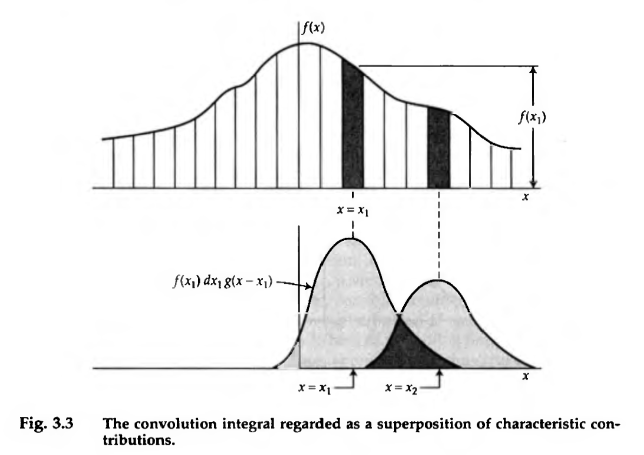
Convolution can also be thought of as a superposition of characteristic contributions. I.e., the final function \(h(x)\) has grabbed value from nearby regions of \(f(x)\), modulated by the envelope of \(g(x)\). This paradigm is very useful for understanding interpolation, smoothing, and kernel density estimation (KDE). Credit: Bracewell Ch. 3
Convolution is commutative
$$ f * g = g * f $$
and associative
$$ f * (g * h) = (f * g) * h $$
and distributive over addition
$$ f * (g + h) = f * g + f * h. $$
It is a linear operator, just like the Fourier transform.
The impulse symbol
We’ll develop a notation for an intense (unit-area) pulse so brief that the measuring equipment is unable to distinguish it from pulses yet briefer still. You may be quite familiar with this concept as a “delta-function,” especially in the context of quantum physics. Physically speaking, things like “point masses”, “point charges,” and (astrophysically speaking) “point sources” do not physically exist, but they are very useful concepts. The only important attribute of an impulse is how it reacts under integration
- \(\delta(x) = 0\) for \(x \ne 0\)
- \(\int_{-\infty}^\infty \delta(x)\,\mathrm{d}x = 1\)
And, there is a close relationship between the impulse symbol and the unit step function \(H(x)\) such that $$ \int_{-\infty}^x \delta(x^\prime)\,\mathrm{d}x^\prime = H(x). $$
Another very important property of the impulse function is its “sifting property” (TMS A2.11), such that $$ f(a) = \int_{-\infty}^{\infty} f(x) \delta(x - a)\,\mathrm{d}x^\prime. $$ i.e., the integral of function \(f(x)\) times a delta-function located at \(a\) will give the value of the function evaluated at \(a\), \(f(a)\).
The Fourier transform of a delta function (centered on 0) is
$$ F(s) = \int_{-\infty}^{\infty} \delta(0) \exp (-i 2 \pi x s)\,\mathrm{d}x = 1. $$ This is yet another important Fourier pair $$ \delta(x) \leftrightharpoons \mathrm{constant\;amplitude\,\forall\, s}. $$
The Sampling or Replicating Symbol “Shah function”
This is an infinite sequence of unit impulses, given by $$ \mathrm{shah}(x) = \sum_{n=-\infty}^\infty \delta(x - n) $$
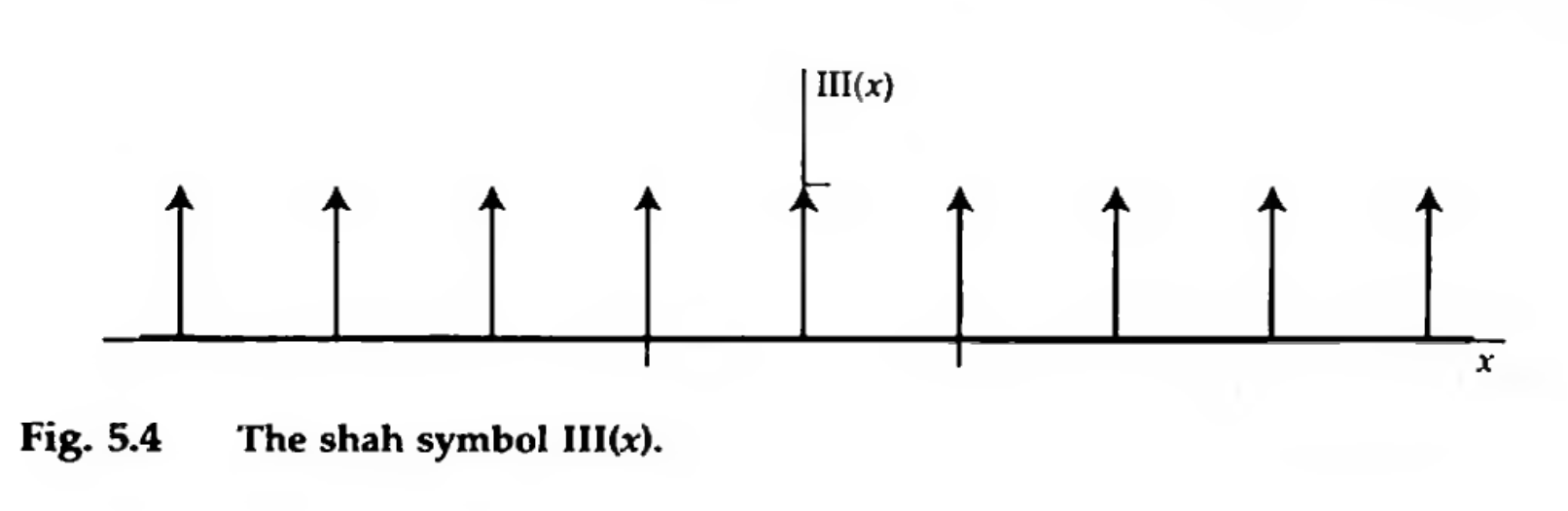
The replicating function. Credit: Bracewell Fig 5.4
Also sometimes called a “Dirac Comb.” There is a generalization of the sifting property, such that if you multiply a function by a shah, you are effectively sampling it at unit intervals.
You can use it to sample \(f(x)\) (by multiplication)
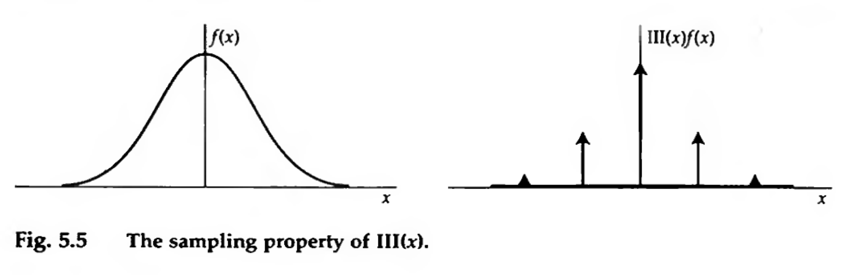
Sampling property of the shah function by multiplication. Credit: Bracewell Fig 5.5
And you can use it to replicate \(f(x)\) (by convolution)
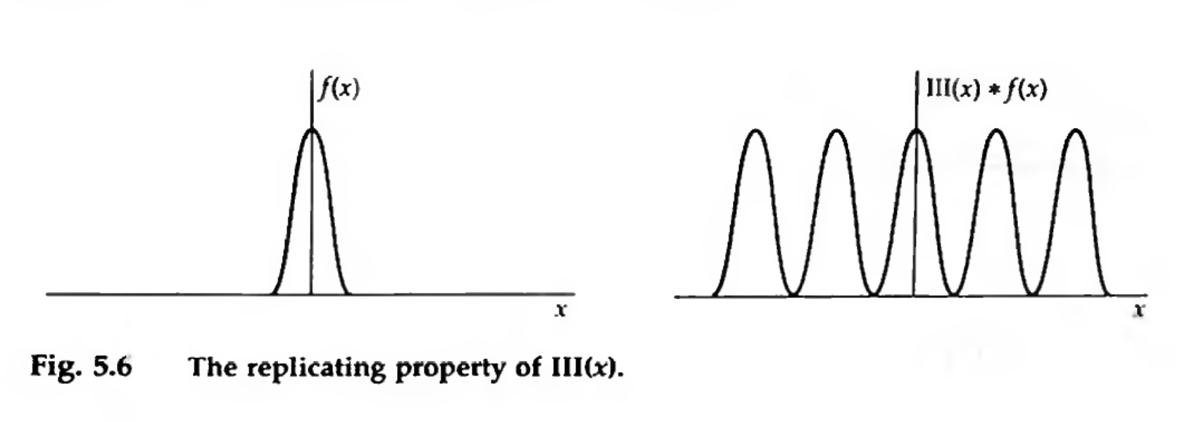
Replicating property of the shah function by convolution. Credit: Bracewell Fig 5.6
The unit shah function is also its own Fourier transform $$ \mathrm{shah}(x) \leftrightharpoons \mathrm{shah}(s) $$
Fourier transform theorems properties: similarity, convolution, multiplication
There are several useful properties of the Fourier transform that you’ll want to familiarize yourself with. See Bracewell Ch. 6 or TMS A2.1.2.
Similarity
If
$$ f(x) \leftrightharpoons F(s) $$
then
$$ f(ax) \leftrightharpoons \frac{1}{|a|} F \left (\frac{s}{a} \right). $$
I.e., applied to waveforms and spectra, a compression of the time scale corresponds to an expansion of the frequency scale.
Fourier transforms and the Heisenberg uncertainty principle
In a signal-processing sense, this manifests as an inability to precisely specify a signal in both the time and frequency domains at the same time. As you decrease the variance of a function (i.e., make it more concentrated and thus localized) in one domain, you increase the variance of it in the other domain (i.e., make it more extended and thus dispersed).
In quantum mechanics, this same concept is at play in the Heisenberg Uncertainty principle, where probability distributions (i.e., wavefunctions) governing position and momentum are related by the Fourier transform. It’s impossible to know both position and momentum precisely.
Shift
If
$$ f(x) \leftrightharpoons F(s) $$
then
$$ f(x - a) \leftrightharpoons \exp(- 2 \pi i a s) F(s). $$
If you shift a function, then there are no changes in the amplitude of the Fourier transform, but, there are changes to its phase, dependent on s. The higher the frequency, the greater the change in phase angle. In radio astronomy, it’s common to hear of this as a translation in the R.A./Dec. plane results in a phase shift in the visibility plane.